Elliott Z. Stein, a senior litigation strategist at Bloomberg Intelligence, shared his opinion on why leading American crypto exchange Coinbase has a good chance of securing victory in its motion to dismiss all claims made against it by the U.S. Securities and Exchange Commission (SEC).
OnnxStream is an open-source project created by Vito Plantamura with the original intention of running Stable Diffusion 1.5 (SD1.5) on a Raspberry Pi Zero 2 by minimising memory consumption as much as possible, albeit at the cost of increased inference latency/throughput.
At the time of writing, it has expanded to support not only Stable Diffusion 1.5 but also Stable Diffusion XL 1.0 Base (SDXL) and Stable Diffusion XL Turbo 1.0. I won’t go into detail about how exactly this amazing feat is being achieved since the GitHub repository already explains it very well.
Instead, let’s just jump right into getting it working.
Technical Requirements
All you need is the following:
Raspberry Pi 5 — Or Raspberry Pi 4 or any other Raspberry Pi, just expect it to be slower
SD Card — Minimally 16GB, with Raspbian or some Linux distro already setup. The SDXL Turbo weights are around 8GB.
An internet connection
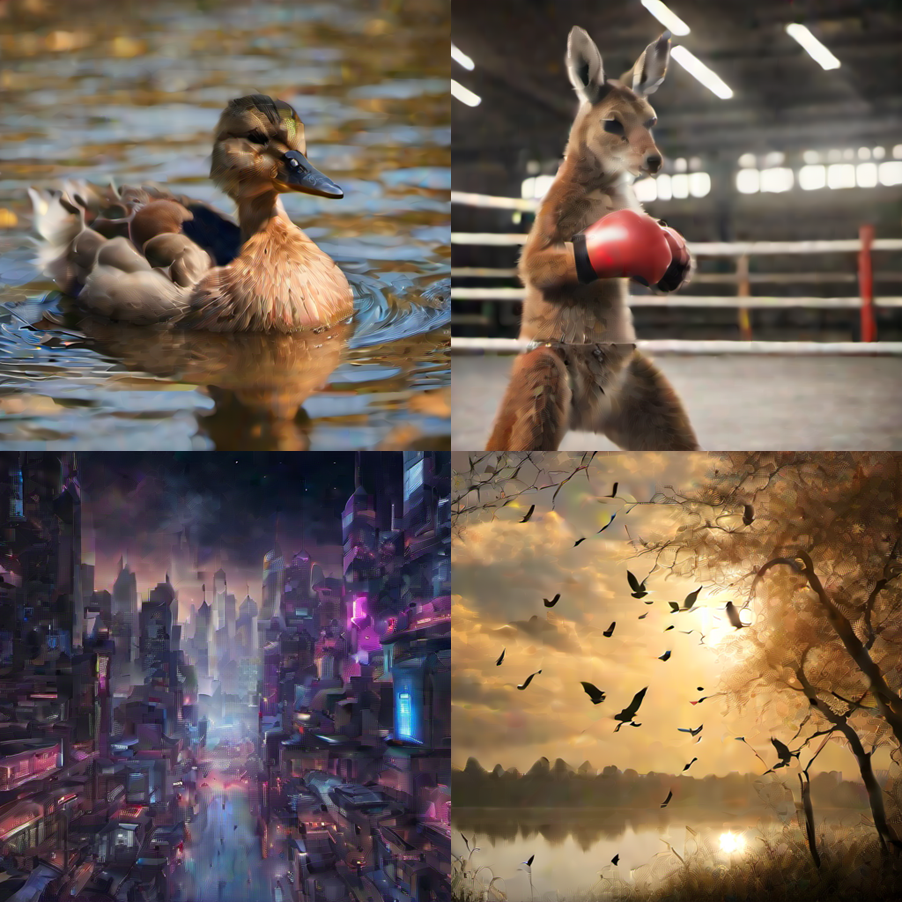
Images generated in a single diffusion step on the Raspberry Pi | Source: Author
Setting Up OnnxStream
The instructions here are from the GitHub repository, but I’m breaking it down and explaining it a bit more.
1. Building XNNPack
First, we have to install XNNPack, which is a library from Google that provides “high-efficiency floating-point neural network inference operators”. But we can’t just get the latest version in case of any breaking changes. Instead, we shall get the version that the OnnxStream creator has verified to be working at the time of writing. In a terminal, run:
XNNPack will take a couple of minutes to build. Go get coffee or something.
2. Building OnnxStream
Next, we have to build OnnxStream. In a terminal, run:
git clone https://github.com/vitoplantamura/OnnxStream.git
cd OnnxStream
cd src
mkdir build
cd build
cmake -DMAX_SPEED=ON -DXNNPACK_DIR=<DIRECTORY_WHERE_XNNPACK_WAS_CLONED> ..
cmake --build . --config Release
Make sure to replace <DIRECTORY_WHERE_XNNPACK_WAS_CLONED> with the path at which XNNPack was cloned to (not the build folder). In my case, it was at /home/admin/XNNPACK/.
3. Downloading Model Weights
Now, we need to download the model weights for SDXL Turbo. In a terminal, run:
If you have not installed git-lfs yet, do so first. This will take even longer than the step before since the model weights are quite big. Go get lunch!
You can also run the other two models supported — Stable Diffusion 1.5 and Stable Diffusion XL 1.0 Base by downloading their weights from the links provided in OnnxStream’s GitHub repository. Make sure your SD card has enough space if you are downloading all these models!
Once done, that’s it! We are ready to generate images on a Raspberry Pi!
Generating Images
To generate images, run the code block below:
cd ~/OnnxStream/src/build/
./sd --turbo --models-path /home/admin/stable-diffusion-xl-turbo-1.0-onnxstream --prompt "An astronaut riding a horse on Mars" --steps 1 --output astronaut.png
Replace the prompt with what you want to generate. I’m just using the go-to classic astronaut prompt here. I set steps to just 1 as SDXL Turbo doesn’t need many steps to generate a good-looking image.
There are other arguments you can pass too, such as — neg-prompt for negative prompts (SDXL Turbo does not support negative prompts but you can use it for the other two models), — steps to set the number of generative steps and — seed to set the random seed.
The arguments required will change according to the type of model used, so please take a look at OnnxStream’s GitHub repository for the full list of arguments to pass if you’re using something other than SDXL Turbo.
You should get an output like this | Source: Author
As you can see in the image above, on the Raspberry Pi 5, each diffusion step takes around 1 minute, and in total with pre-processing and decoding, it around 3 minutes to generate a single image.
Image with 1, 2, 5, and 10 steps respectively, using the same seed and prompt | Source: Author
Here’s a comparison and progression of the same prompt with the same seed from step 1 to 10. You can see that even with a single step with refinement, the generated image is already really well-done. This is in contrast to SDXL or SD1.5 which requires quite a few steps to reach that quality.
Conclusion
With it taking around at least a couple of minutes to generate an image, the question of use cases for it comes begging.
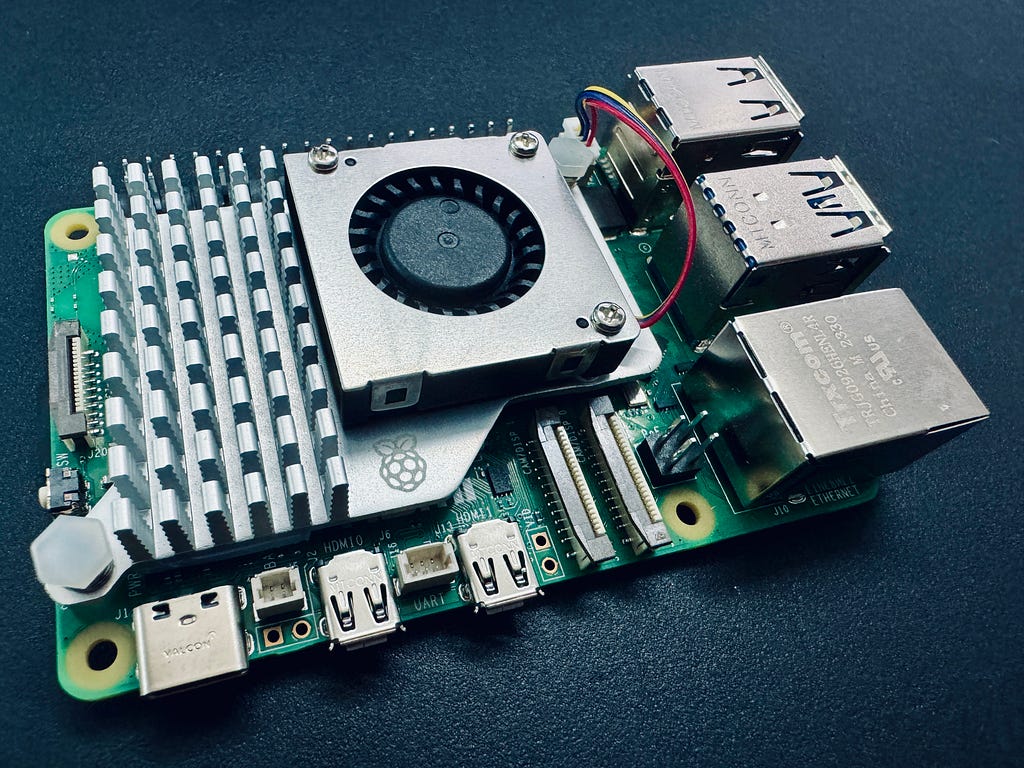
Obligatory shot of my Raspberry Pi 5 | Source: Author
The most obvious and fun use case to me is an ever-changing photo frame that will generate a new image every few minutes. There is actually a project along this tangent that uses OnnxStream, by rvdveen on GitHub, where he uses OnnxStream on a Raspberry Pi Zero 2 W to generate images for news articles and shows it on a photo frame using an e-ink display. It takes around 5 hours to generate an image on the Pi Zero 2 W with what should be SD1.5, but hey it’s not like you need a photo frame to be changing what it’s showing in real-time.
Or maybe you just want your own locally hosted image generator which can produce decent quality images while not hogging any major compute devices on your network.
Have fun playing around with SDXL Turbo on the Raspberry Pi!
Disclaimer: I have no affiliation with OnnxStream or StabilityAI. All views and opinions are my own and do not represent any organisation.
Is being able to build and train machine learning models from popular libraries sufficient for machine learning users? Probably not for too long. With tools like AutoAI on the rise, it is likely that a lot of the very traditional machine learning skills like building model architectures with common libraries like Pytorch will be less important.
What is likely to persist is the demand for skilled users with a deep understanding of the underlying principles of ML, particularly in problems that require novel challenges, customisation, optimisation. To be more innovative and novel, it is important to have a deep understanding of the mathematical foundations of these algorithms. In this article, we’ll look at the mathematical description of one such important model, Recurrent Neural Network (RNN).
Time series data (or any sequential data like language) has a temporal dependencies and is widespread across various sectors ranging from weather prediction to medical applications. RNN is a powerful tool for capturing sequential patterns in such data. In this article, we’ll delve into the mathematical foundations of RNNs and implement these equations from scratch using python.
Understanding RNNs: The Mathematical Description
An important element of sequential data is the temporal dependence where the past values determine the current and future values (just like the predetermined world we live in but let’s not get philosophical and stick to RNN models). Time series forecasting utilises this nature of sequential data and focuses on the prediction of the next value given previous n values. Depending on the model, this includes either mapping or regression of the past values.
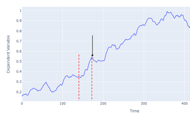
Figure 1. An example of a time series data
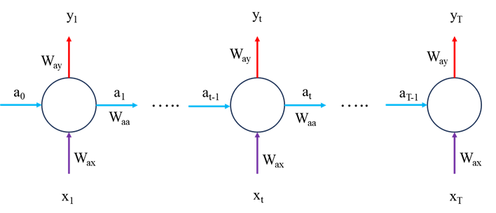
Consider the point indicated with the black arrow, y and the points before y (between the red dashed line) denoting as X = {x1 , x2 , ….xt …..xT} where T is the total number of time steps. The RNN processes the input sequence (X) by placing each input through a hidden state (or sometimes refered to as memory state) and outputs y. These hidden states allow the model to capture and remember patterns from earlier points in the sequence.
Figure 2. A schematic of an RNN model, showing the inputs, hidden states and outputs
Now let’s look at the mathematical operations within the RNN model, first lets consider the forward pass, we’ll worry about the model optimisation later.
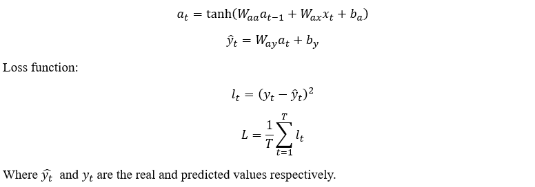
Forward Pass
The forward pass is fairly straightforward and is as follows:
Backpropagation Through Time
In machine learning, the optimisation (variable updates) are done using the gradient descent method:
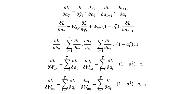
Therefore, all parameters that need updating during training will require their partial derivatives. Here we’ll derive the partial derivative of the loss function with respect to each variable included in the forward pass equations:
By noting the forward pass equations and network schematic in Figure 2, we can see that at time T, L only depends on a_T via y_T i.e.
However, for t < T, L depends on a_T via y_T and a_(T+1) so let’s use the chain rule for both:
Now we have the equations for the gradient of the loss function with respect all parameters present in the forward pass equation. This algorithm is called Backpropagation Through Time. It is important to clarify that for a time series data, usually only the last value contribute to the Loss function i.e. all other outputs are ignored and their contribution to the loss function set to 0. The mathematical description is the same as that presented. Now Let’s code these equations in python and apply it to an example dataset.
The Coding Implementation
Before we can implement the equations above, we’ll need to import the necessary dataset, preprocess and ready for the model training. All of this work is very standard in any time series analysis.
import numpy as np import pandas as pd import matplotlib.pyplot as plt import plotly.graph_objs as go from plotly.offline import iplot import yfinance as yf import datetime as dt import math
#### Data Processing start_date = dt.datetime(2020,4,1) end_date = dt.datetime(2023,4,1)
#loading from yahoo finance data = yf.download("GOOGL",start_date, end_date)
The model Now we implement the mathematical equations. it is definitely worth reading through the code, noting the dimensions of all variables and respective derivates to give yourself a better understanding of these equations.
class SimpleRNN: def __init__(self,input_dim,output_dim, hidden_dim): self.input_dim = input_dim self.output_dim = output_dim self.hidden_dim = hidden_dim self.Waa = np.random.randn(hidden_dim, hidden_dim) * 0.01 # we initialise as non-zero to help with training later self.Wax = np.random.randn(hidden_dim, input_dim) * 0.01 self.Way = np.random.randn(output_dim, hidden_dim) * 0.01 self.ba = np.zeros((hidden_dim, 1)) self.by = 0 # a single value shared over all outputs #np.zeros((hidden_dim, 1))
def FeedForward(self, x): # let's calculate the hidden states a = [np.zeros((self.hidden_dim,1))] y = [] for ii in range(len(x)):
# remove the first a and y values used for initialisation #a = a[1:] return y, a
def ComputeLossFunction(self, y_pred, y_actual): # for a normal many to many model: #loss = np.sum((y_pred - y_actual) ** 2) # in our case, we are only using the last value so we expect scalar values here rather than a vector loss = (y_pred[-1] - y_actual) ** 2 return loss
def predict(self, x, n, a_training): # let's calculate the hidden states a_future = a_training y_predict = []
# Predict the next n terms for ii in range(n): a_next = np.tanh(np.dot(self.Waa, a_future[-1]) + np.dot(self.Wax, x[ii]) + self.ba) a.append(a_next) y_predict.append(np.dot(self.Way, a_next) + self.by)
return y_predict
Training and Testing the model
input_dim = 1 output_dim = 1 hidden_dim = 50
learning_rate = 1e-3
# Initialize The RNN model rnn_model = SimpleRNN(input_dim, output_dim, hidden_dim)
# train the model for 200 epochs
for epoch in range(200): for ii in range(len(X_train)): y_pred, a = rnn_model.FeedForward(X_train[ii]) loss = rnn_model.ComputeLossFunction(y_pred, y_train[ii]) dLdy, dLdby, dLdWay, dLdWax, dLdWaa, dLdba = rnn_model.ComputeGradients(a, X_train[ii], y_pred, y_train[ii]) rnn_model.UpdateParameters(dLdby, dLdWay, dLdWax, dLdWaa, dLdba, learning_rate) print(f'Loss: {loss}')
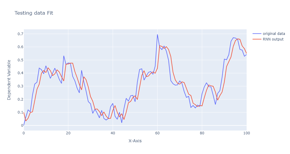
y_test_predicted = [] for jj in range(len(X_test)): forecasted_values, _ = rnn_model.FeedForward(X_test[jj]) y_test_predicted.append(forecasted_values[-1])
y_test_predicted_flat = np.array([val[0, 0] for val in y_test_predicted]) trace1 = go.Scatter(y = y_test.ravel(), mode ="lines", name = "original data") trace2 = go.Scatter(y=y_test_predicted_flat, mode = "lines", name = "RNN output") layout = go.Layout(title='Testing data Fit', xaxis=dict(title='X-Axis'), yaxis=dict(title='Dependent Variable')) figure = go.Figure(data = [trace1,trace2], layout = layout)
iplot(figure)
That brings us to the end of this demonstration but hopefully only the start of your reading into these powerful models. You might find it helpful to test your understanding by experimenting with a different activation function in the forward pass. Or read further into sequential models like LSTM and transformers which are formidable tools, especially in language-related tasks. Exploring these models can deepen your understanding of more sophisticated mechanisms for handling temporal dependencies. Finally, thank you for taking the time to read this article, I hope you found it useful in your understanding of RNN or their mathematical background.
Unless otherwise noted, all images are by the author
Today’s top deals include 50% off an Anker PowerExpand 12-in-1 media dock, 14% off an Apple Magic Mouse, 50% off Apple Watch Series 6, 56% off a Shark 3-in-1 Clean Sense HEPA air purifier, and more.
Save $200 on an M3 Pro MacBook Pro
The AppleInsider staff scours the web for amazing deals at online stores to showcase a list of deep discounts on trending tech gadgets, including deals on Apple Watches, TVs, accessories, and other products. We post the hottest deals daily to help you save money.
We use cookies on our website to give you the most relevant experience by remembering your preferences and repeat visits. By clicking “Accept”, you consent to the use of ALL the cookies.
This website uses cookies to improve your experience while you navigate through the website. Out of these, the cookies that are categorized as necessary are stored on your browser as they are essential for the working of basic functionalities of the website. We also use third-party cookies that help us analyze and understand how you use this website. These cookies will be stored in your browser only with your consent. You also have the option to opt-out of these cookies. But opting out of some of these cookies may affect your browsing experience.
Necessary cookies are absolutely essential for the website to function properly. These cookies ensure basic functionalities and security features of the website, anonymously.
Cookie
Duration
Description
cookielawinfo-checkbox-analytics
11 months
This cookie is set by GDPR Cookie Consent plugin. The cookie is used to store the user consent for the cookies in the category "Analytics".
cookielawinfo-checkbox-functional
11 months
The cookie is set by GDPR cookie consent to record the user consent for the cookies in the category "Functional".
cookielawinfo-checkbox-necessary
11 months
This cookie is set by GDPR Cookie Consent plugin. The cookies is used to store the user consent for the cookies in the category "Necessary".
cookielawinfo-checkbox-others
11 months
This cookie is set by GDPR Cookie Consent plugin. The cookie is used to store the user consent for the cookies in the category "Other.
cookielawinfo-checkbox-performance
11 months
This cookie is set by GDPR Cookie Consent plugin. The cookie is used to store the user consent for the cookies in the category "Performance".
viewed_cookie_policy
11 months
The cookie is set by the GDPR Cookie Consent plugin and is used to store whether or not user has consented to the use of cookies. It does not store any personal data.
Functional cookies help to perform certain functionalities like sharing the content of the website on social media platforms, collect feedbacks, and other third-party features.
Performance cookies are used to understand and analyze the key performance indexes of the website which helps in delivering a better user experience for the visitors.
Analytical cookies are used to understand how visitors interact with the website. These cookies help provide information on metrics the number of visitors, bounce rate, traffic source, etc.
Advertisement cookies are used to provide visitors with relevant ads and marketing campaigns. These cookies track visitors across websites and collect information to provide customized ads.