Keep your gear topped up and your favorite items in one place with the handy Mag:3 Classics Device Charging Tray, featuring MagSafe charging, Qi charging, and a bonus USB-C port.
Mag:3 Classics Device Charging Tray
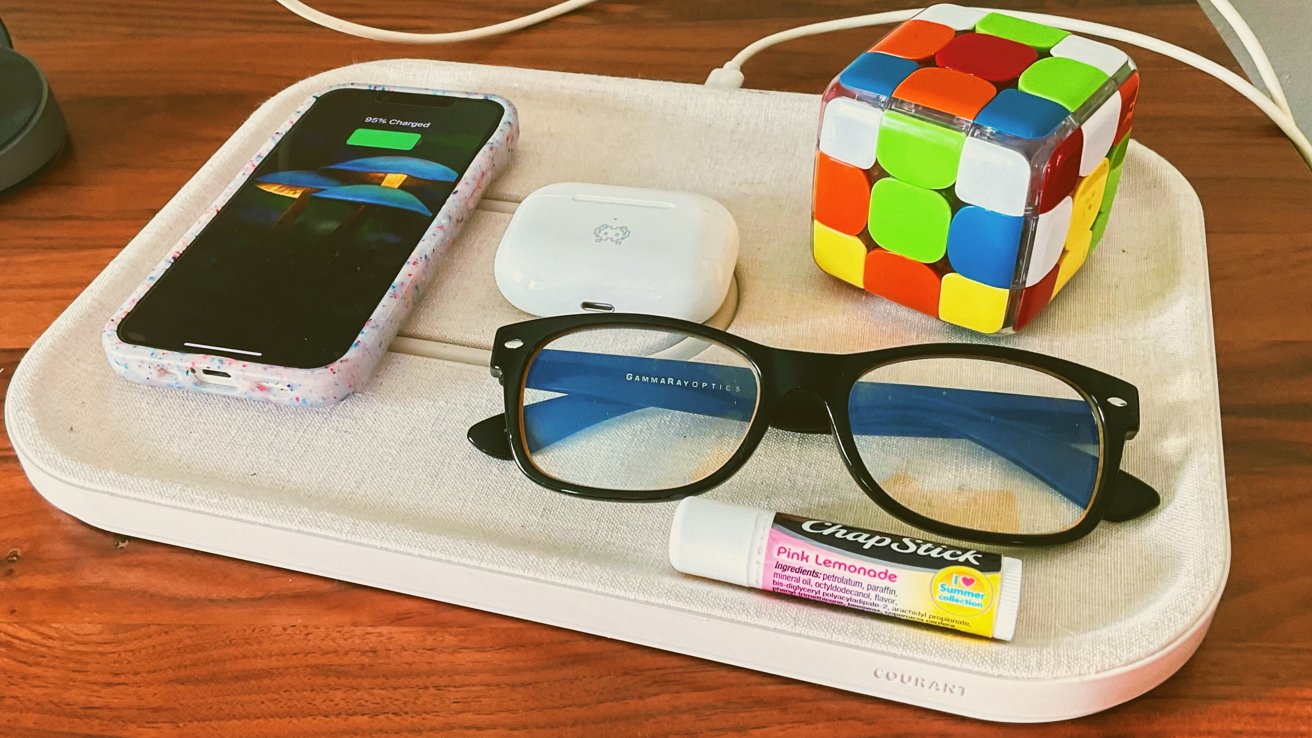
If you’re like us, you probably stuff your iPhone and AirPods into your pockets, purse, or bag before leaving your house in the morning and decant them somewhere at day’s end. However, unless you have a dedicated place for your gear, misplacing one of your much-loved items is pretty easy.
Courant’s Mag:3 Classics Device Charging Tray aims to fix that. It features multiple ways to charge your favorite gear in a handy tray that keeps all your everyday carry items in the same place.
The driving force behind this explosive growth seems to be intertwined with the launch of Xpayments, which left the cryptocurrency community buzzing with speculation.
Learn how a neural network with one hidden layer using ReLU activation can represent any continuous nonlinear functions.
Activation functions play an integral role in Neural Networks (NNs) since they introduce non-linearity and allow the network to learn more complex features and functions than just a linear regression. One of the most commonly used activation functions is Rectified Linear Unit (ReLU), which has been theoretically shown to enable NNs to approximate a wide range of continuous functions, making them powerful function approximators.
In this post, we study in particular the approximation of Continuous NonLinear (CNL) functions, the main purpose of using a NN over a simple linear regression model. More precisely, we investigate 2 sub-categories of CNL functions: Continuous PieceWise Linear (CPWL), and Continuous Curve (CC) functions. We will show how these two function types can be represented using a NN that consists of one hidden layer, given enough neurons with ReLU activation.
For illustrative purposes, we consider only single feature inputs yet the idea applies to multiple feature inputs as well.
ReLU activation
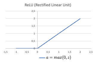
Figure 1: Rectified Linear Unit (ReLU) function.
ReLU is a piecewise linear function that consists of two linear pieces: one that cuts off negative values where the output is zero, and one that provides a continuous linear mapping for non negative values.
Continuous piecewise linear function approximation
CPWL functions are continuous functions with multiple linear portions. The slope is consistent on each portion, than changes abruptly at transition points by adding new linear functions.
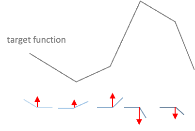
Figure 2: Example of CPWL function approximation using NN. At each transition point, a new ReLU function is added to/subtracted from the input to increase/decrease the slope.
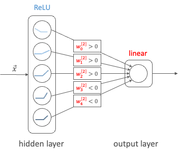
In a NN with one hidden layer using ReLU activation and a linear output layer, the activations are aggregated to form the CPWL target function. Each unit of the hidden layer is responsible for a linear piece. At each unit, a new ReLU function that corresponds to the changing of slope is added to produce the new slope (cf. Fig.2). Since this activation function is always positive, the weights of the output layer corresponding to units that increase the slope will be positive, and conversely, the weights corresponding to units that decreases the slope will be negative (cf. Fig.3). The new function is added at the transition point but does not contribute to the resulting function prior to (and sometimes after) that point due to the disabling range of the ReLU activation function.
Figure 3: Approximation of the CPWL target function in Fig.2 using a NN that consists of one hidden layer with ReLU activation and a linear output layer.
Example
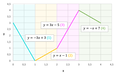
To make it more concrete, we consider an example of a CPWL function that consists of 4 linear segments defined as below.
Figure 4: Example of a PWL function.
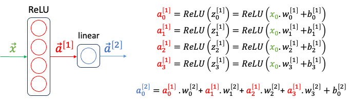
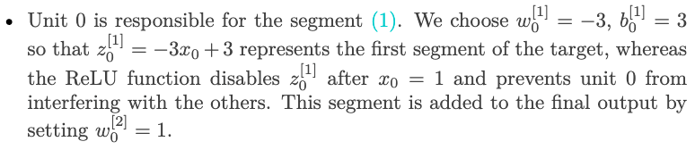
To represent this target function, we will use a NN with 1 hidden layer of 4 units and a linear layer that outputs the weighted sum of the previous layer’s activation outputs. Let’s determine the network’s parameters so that each unit in the hidden layer represents a segment of the target. For the sake of this example, the bias of the output layer (b2_0) is set to 0.
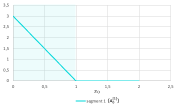
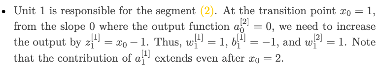
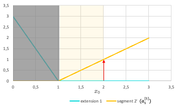
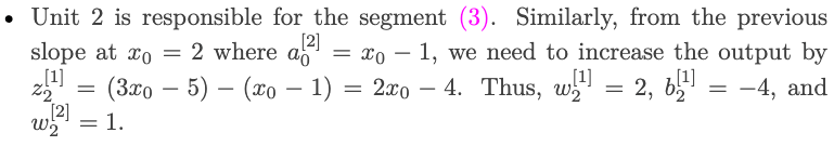
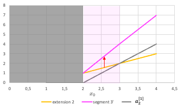
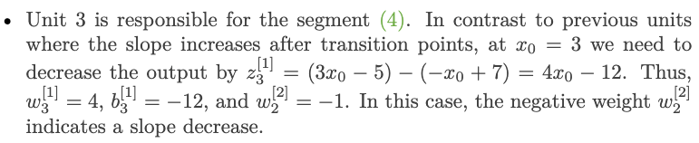
Figure 5: The network architecture to model the PWL function defined in Fig.4.Figure 6: The activation output of unit 0 (a1_0).Figure 7: The activation output of unit 1 (a1_1), which is aggregated to the output (a2_0) to produce the segment (2). The red arrow represents the change in slope.Figure 8: The output of unit 2 (a1_2), which is aggregated to the output (a2_0) to produce the segment (3). The red arrow represents the change in slope.Figure 9: The output of unit 3 (a1_3), which is aggregated to the output (a2_0) to produce the segment (4). The red arrow represents the change in slope.
Continuous curve function approximation
The next type of continuous nonlinear function that we will study is CC function. There is not a proper definition for this sub-category, but an informal way to define CC functions is continuous nonlinear functions that are not piecewise linear. Several examples of CC functions are: quadratic function, exponential function, sinus function, etc.
A CC function can be approximated by a series of infinitesimal linear pieces, which is called a piecewise linear approximation of the function. The greater the number of linear pieces and the smaller the size of each segment, the better the approximation is to the target function. Thus, the same network architecture as previously with a large enough number of hidden units can yield good approximation for a curve function.
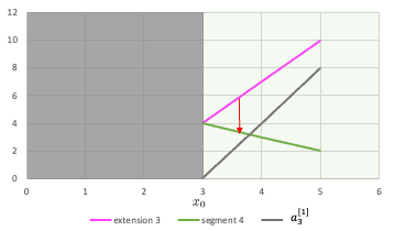
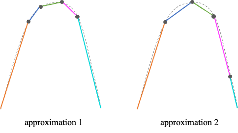
However, in reality, the network is trained to fit a given dataset where the input-output mapping function is unknown. An architecture with too many neurons is prone to overfitting, high variance, and requires more time to train. Therefore, an appropriate number of hidden units must not be too small to properly fit the data, nor too large to lead to overfitting. Moreover, with a limited number of neurons, a good approximation with low loss has more transition points in restricted domain, rather than equidistant transition points in an uniform sampling way (as shown in Fig.10).
Figure 10: Two piecewise linear approximations for a continuous curve function (in dashed line). The approximation 1 has more transition points in restricted domain and model the target function better than the approximation 2.
Wrap up
In this post, we have studied how ReLU activation function allows multiple units to contribute to the resulting function without interfering, thus enables continuous nonlinear function approximation. In addition, we have discussed about the choice of network architecture and number of hidden units in order to obtain a good approximation result.
I hope that this post is useful for your Machine Learning learning process!
Further questions to think about:
How does the approximation ability change if the number of hidden layers with ReLU activation increase?
How ReLU activations are used for a classification problem?
*Unless otherwise noted, all images are by the author
We use cookies on our website to give you the most relevant experience by remembering your preferences and repeat visits. By clicking “Accept”, you consent to the use of ALL the cookies.
This website uses cookies to improve your experience while you navigate through the website. Out of these, the cookies that are categorized as necessary are stored on your browser as they are essential for the working of basic functionalities of the website. We also use third-party cookies that help us analyze and understand how you use this website. These cookies will be stored in your browser only with your consent. You also have the option to opt-out of these cookies. But opting out of some of these cookies may affect your browsing experience.
Necessary cookies are absolutely essential for the website to function properly. These cookies ensure basic functionalities and security features of the website, anonymously.
Cookie
Duration
Description
cookielawinfo-checkbox-analytics
11 months
This cookie is set by GDPR Cookie Consent plugin. The cookie is used to store the user consent for the cookies in the category "Analytics".
cookielawinfo-checkbox-functional
11 months
The cookie is set by GDPR cookie consent to record the user consent for the cookies in the category "Functional".
cookielawinfo-checkbox-necessary
11 months
This cookie is set by GDPR Cookie Consent plugin. The cookies is used to store the user consent for the cookies in the category "Necessary".
cookielawinfo-checkbox-others
11 months
This cookie is set by GDPR Cookie Consent plugin. The cookie is used to store the user consent for the cookies in the category "Other.
cookielawinfo-checkbox-performance
11 months
This cookie is set by GDPR Cookie Consent plugin. The cookie is used to store the user consent for the cookies in the category "Performance".
viewed_cookie_policy
11 months
The cookie is set by the GDPR Cookie Consent plugin and is used to store whether or not user has consented to the use of cookies. It does not store any personal data.
Functional cookies help to perform certain functionalities like sharing the content of the website on social media platforms, collect feedbacks, and other third-party features.
Performance cookies are used to understand and analyze the key performance indexes of the website which helps in delivering a better user experience for the visitors.
Analytical cookies are used to understand how visitors interact with the website. These cookies help provide information on metrics the number of visitors, bounce rate, traffic source, etc.
Advertisement cookies are used to provide visitors with relevant ads and marketing campaigns. These cookies track visitors across websites and collect information to provide customized ads.