A nonlinear correlation measure for your everyday tasks

Traditional correlation coefficients such as Pearson ρ, Spearman, or Kendall’s τ are limited to finding linear or monotonic relationships and struggle to identify more complex association structures. The recent article on TDS [1] about a new correlation coefficient ξ that aims to overcome these limitations has received a lot of attention and has been discussed intensively. One of the questions raised in the comments was what particular advantages ξ brings over a nonlinear correlation measure based on mutual information. An experiment may be worth a thousand words in such debates. So in this story, I experimentally compare ξ to the mutual information-based coefficient R along a variety of properties one would like a nonlinear correlation measure to satisfy. Based on the results, I would strongly recommend R over ξ for the majority of routines that require finding nonlinear associations.
Requirements
Let me first summarize and convince you about the desired properties of a coefficient we are looking for. We want an association measure A(x,y) that
- is nonlinear. That is, it takes the value zero when x and y are independent; it has a value of one for the modulus of the measure when there is an exact nonlinear relationship between the variables, such as x = h(t), y=f(t), where t is a parameter;
- is symmetric. That is, A(x,y)=A(y,x). The opposite would be confusing;
- is consistent. That is, it is equal to the linear correlation coefficient ρ when x, y have a bivariate normal distribution, i.e. is a generalization of ρ to other distributions. This is because ρ is widely used in practice, and many of us have developed a sense of how its values relate to the strength of the relationship. In addition, ρ has a clear meaning for a standard normal distribution, since it completely defines it;
- is scalable — one can compute correlations even for datasets with many observations in a reasonable time;
- is precise, i.e., has a low variance estimator.
The table below summarizes the results of my experiments, where green indicates that the measure has the property tested, red indicates the opposite, and orange is slightly better than red. Let me now walk you through the experiments; you can find their code in this Github repo [2] in the R programming language.

Coefficients of correlation
I use the following coefficient implementations and their configurations
- For the linear correlation coefficient ρ, I use the standard function cor() from the ‘stats’ package;
- for ξ, I use the xicor()function from the ‘XICOR’ package [3];
- mutual information (MI) takes values in the range [0,∞) and there are several ways to estimate it. Therefore, for R one has to choose (a) the MI estimator to use and (b) the transformation to bring MI into the range [0,1].
There are histogram-based and nearest neighbor-based MI estimators. Although many still use histogram-based estimators, I believe that Kraskov’s nearest neighbor estimator [4] is one of the best. I will use its implementation mutinfo() from the ‘FNN’ package [5] with the parameter k=2 as suggested in the paper.
Write in the comments if you want to know more about this particular MI estimator
There are also several ways to normalize the MI to the interval [0,1]. I will use the one below because it has been shown to have a consistency property, and I will demonstrate it in the experiments.

This measure R is called the Mutual Information Coefficient [6]. However, I have noticed a tendency to confuse it with the more recent Maximal Information Coefficient (MIC) [7]. The latter has been shown to be worse than some alternatives [8], and to lack some of the properties it is supposed to have [9].
Nonlinearity
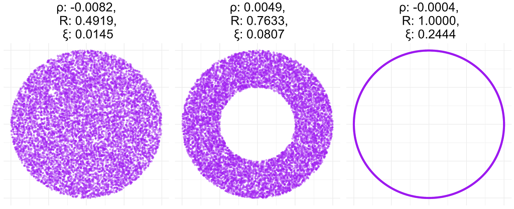
In the figure below, I have calculated all three correlation coefficients for a donut data of 10K points with different donut thickness. As expected, the linear correlation coefficient ρ does not capture the existence of a relationship in any of the plots. In contrast, R correctly determines that x and y are related and takes the value of 1 for the data in the right plot which corresponds to a noiseless relationship between x and y: x = cos(t) and y = sin(t). However, the coefficient ξ is only 0.24 in the latter case. More importantly, in the left plot, ξ is close to zero, even though x and y are not independent.

Symmetry
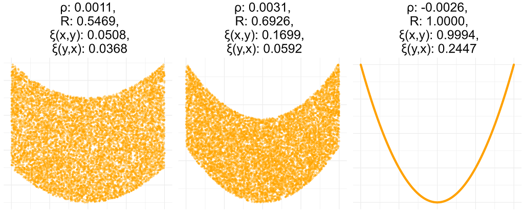
In the figure below, I calculated these quantities for data sets generated from a different distribution. I obtained ρ(x,y)=ρ(y,x) and R(x,y)=R(y,x), so I report only a single value for these measures. However, ξ(x,y) and ξ(y,x) are very different. This is probably due to the fact that y=f(x), but x is not a function of y. This behavior may not be desirable in reality, since it is not easy to interpret a non-symmetric correlation matrix.

Consistency
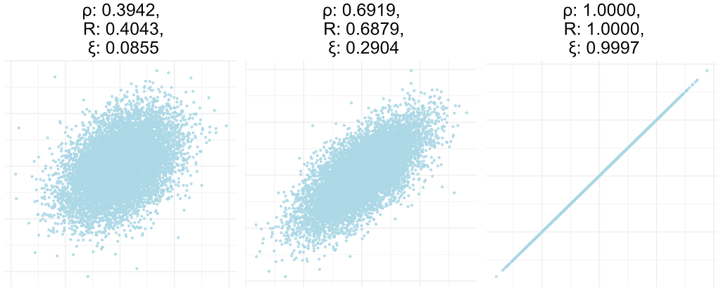
In this experiment, I computed all coefficients for data sets resulting from a bivariate standard normal distribution with a given correlation coefficient of 0.4, 0.7, or 1. Both ρ and R are close to the true correlation, while ξ is not, i.e. it does not have the consistency property defined above.

Scalability
To check the performance of the estimators, I generated data sets of different sizes consisting of two independent and uniformly distributed variables. The figure below shows the time in milliseconds required to compute each coefficient. When the dataset consists of 50K points, R is about 1000 times slower than ξ and about 10000 times slower than ρ. However, it still takes ~10 seconds to compute, which is reasonable when computing a moderate number of correlations. Given the advantages of R discussed above, I’d suggest using it even for computing large numbers of correlations — just subsample your data randomly to ~10K points, where computing R takes less than a second.

Precision
For different samples from the same distribution, there will be different estimates of the correlation coefficient. If there is an association between x and y, we want the variance of these estimates to be small compared to the mean of the correlation. For a measure A(x,y) one can compute precision=sd(A)/mean(A), where sd is a standard deviation. Lower values of this quantity are better. The following table contains precision values calculated from a bivariate normal distribution on data sets of different sizes with different values of the correlation between dimensions. ξ is the least precise, while ρ is the most precise.

References
[1] A New Coefficient of Correlation
[4] Kraskov, A., Stögbauer, H., & Grassberger, P. (2004). Estimating mutual information. Physical review E, 69(6), 066138.
[6] Granger, C., & Lin, J. L. (1994). Using the mutual information coefficient to identify lags in nonlinear models. Journal of time series analysis, 15(4), 371–384.
[7] Reshef, D. N., Reshef, Y. A., Finucane, H. K., Grossman, S. R., McVean, G., Turnbaugh, P. J., … & Sabeti, P. C. (2011). Detecting novel associations in large data sets. science, 334(6062), 1518–1524.
[8] Simon, N., & Tibshirani, R. (2014). Comment on” Detecting Novel Associations In Large Data Sets” by Reshef Et Al, Science Dec 16, 2011. arXiv preprint arXiv:1401.7645.
[9] Kinney, J. B., & Atwal, G. S. (2014). Equitability, mutual information, and the maximal information coefficient. Proceedings of the National Academy of Sciences, 111(9), 3354–3359.
An Undeservedly Forgotten Correlation Coefficient was originally published in Towards Data Science on Medium, where people are continuing the conversation by highlighting and responding to this story.
Originally appeared here:
An Undeservedly Forgotten Correlation Coefficient
Go Here to Read this Fast! An Undeservedly Forgotten Correlation Coefficient
