LoRA, DoRA, AdaLoRA, Delta-LoRA, and more variants of low-rank adaptation.

Low-Rank Adaptation (LoRA) can be considered a major breakthrough towards the ability to train large language models for specific tasks efficiently. It is widely used today in many applications and has inspired research on how to improve upon its main ideas to achieve better performance or train models even faster.
In this article, I want to give an overview of some variants of LoRA, that promise to improve LoRAs capabilities in different ways. I will first explain the basic concept of LoRA itself, before presenting LoRA+, VeRA, LoRA-FA, LoRA-drop, AdaLoRA, DoRA, and Delta-LoRA. I will introduce the basic concepts and main ideas each, and show, how these approaches deviate from the original LoRA. I will spare technical details, unless they are important for the basic concepts, and will also not discuss evaluations in detail. For readers interested, I linked the original papers at the end.
Lora
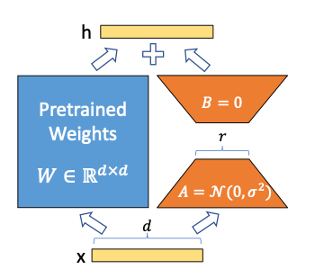
Low-Rank Adaption (LoRA) [1] is a technique, that is widely used today to train large language models (LLMs). Large language models come with the capability to predict tokens of natural language given a natural language input. This is an astonishing capability, but for solving many problems this is not enough. Most of the time, you want to train an LLM on a given downstream task, such as classifying sentences or generating answers to given questions. The most straightforward way of doing that is fine-tuning, where you train some of the layers of the LLM with data of the desired task. That means training very big models with millions to billions of parameters though.
LoRA gives an alternative way of training that is much faster and easier to conduct due to a drastically reduced number of parameters. Next to the parameter weights of an already pre-trained LLM layer, LoRA introduces two matrices A and B, that are called adapters and that are much smaller. If the original matrix of parameters W is of size d x d, the matrices A and B are of size d x r and r x d, where r is much smaller (typically below 100). The parameter r is called the rank. That is, if you use LoRA with a rank of r=16, these matrices are of shape 16 x d. The higher the rank, the more parameters you train. That can lead to better performance on the one hand but needs more computation time on the other.
Now that we have these new matrices A and B, what happens with them? The input fed to W is also given to B*A, and the output of B*A is added to the output of the original matrix W. That is, you train some parameters on top and add their output to the original prediction, which allows you to influence the model’s behavior. You don’t train W anymore, which is why we sometimes say that W is frozen. Importantly, the addition of A and B is not only done at the very end (which would just add a layer on top) but can be applied to layers deep inside the neural network.
That is the main idea of LoRA, and its biggest advantage is, that you have to train fewer parameters than in fine-tuning, but still get comparable performance. One more technical detail I want to mention at this place: At the beginning, the matrix A is initialized with random values of mean zero, but with some variance around that mean. The matrix B is initialized as a matrix of complete zeros. This ensures, that the LoRA matrices don’t change the output of the original W in a random fashion from the very beginning. The update of A and B on W’s output should rather be an addition to the original output, once the parameters of A and B are being tuned in the desired direction. However, we will later see that some approaches deviate from this idea for different reasons.
LoRA as just explained is used very often with today’s LLMs. However, by now there are many variants of LoRA that deviate from the original method in different ways and aim at improving speed, performance, or both. Some of these I want to present to you in the following.
LoRA+
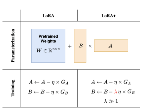
LoRA+ [2] introduces a more efficient way of training LoRA adapters by introducing different learning rates for matrices A and B. Most of the time, when training a neural network, there is just one learning rate that is applied to all weight matrices the same way. However, for the adapter matrices used in LoRA, the authors of LoRA+ can show, that it is suboptimal to have that single learning rate. The training becomes more efficient by setting the learning rate of matrix B much higher than that of matrix A.
There is a theoretical argument to justify that approach, that mainly bases on numerical caveats of a neural network’s initialization if the model becomes very wide in terms of the number of its neurons. However, the math required to prove that is quite complicated (if you are really into it, feel free to take a look at the original paper [2]). Intuitively, you may think that matrix B, which is initialized with zero, could use bigger update steps than the randomly initialized matrix A. In addition, there is empirical evidence for an improvement by that approach. By setting the learning rate of matrix B 16 times higher than that of matrix A, the authors have been able to gain a small improvement in model accuracy (around 2%), while speeding up the training time by factor two for models such as RoBERTa or Llama-7b.
VeRA
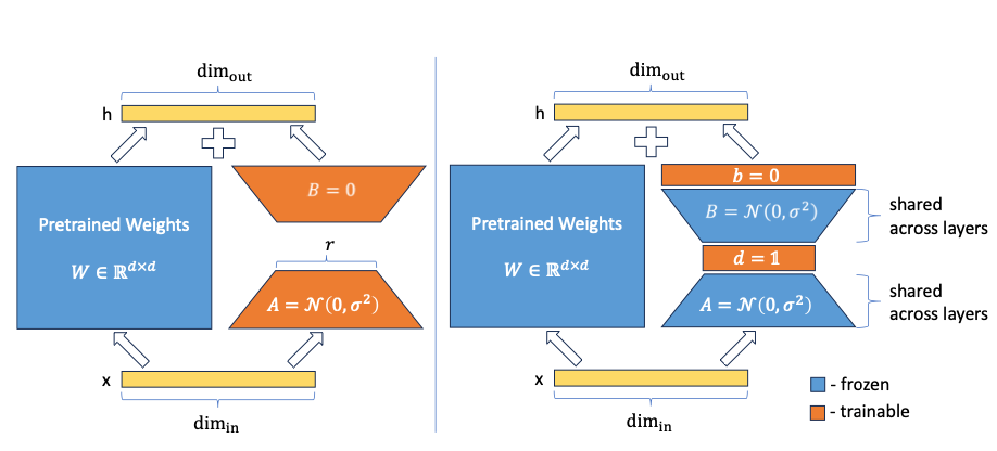
With VeRA (Vector-based Random Matrix Adaptation) [3], the authors introduce an approach to drastically reduce the parameter size of the LoRA adapters. Instead of training the matrices A and B, which is the core idea of LoRA in the first place, they initialize these matrices with shared random weights (i.e. all the matrices A and B in all the layers have the same weights) and add two new vectors d and b. Only these vectors d and b are trained in the following.
You may wonder how this can work at all. A and B are matrices of random weights. How should they contribute anything to the model’s performance, if they are not trained at all? This approach is based on an interesting field of research on so-called random projections. There is quite some research that indicates that in a large neural network only a small fraction of the weights is used to steer the behavior and lead to the desired performance on the task the model was trained for. Due to the random initialization, some parts of the model (or sub-networks) are contributing more towards the desired model behavior from the very beginning. During the training, all parameters are trained though, as it is now known which are the important subnetworks. That makes training very costly, as most of the parameters that are updated don’t add any value to the model’s prediction.
Based on this idea, there are approaches to only train these relevant sub-networks. A similar behavior can be obtained by not training the sub-networks themselves, but by adding projection vectors after the matrix. Due to the multiplication of the matrix with the vector, this can lead to the same output as tuning some sparse parameters in the matrix would. That is exactly what the authors of VeRA propose by introducing the vectors d and b, which are trained, while the matrices A and B are frozen. Also, in contrast to the original LoRa approach, matrix B is not set to zero anymore but is initialized randomly just as matrix A.
This approach naturally leads to a number of parameters that is much smaller than the full matrices A and B. For example, if you introduce LoRA-layers of rank 16 to GPT-3, you would have 75.5M parameters. With VeRA, you only have 2.8M (a reduction of 97%). But how is the performance with such a small number of parameters? The authors of VeRA performed an evaluation with some common benchmarks such as GLUE or E2E and with models based on RoBERTa and GPT2 Medium. Their results suggest, that the VeRA model yields performance that is only marginally lower than models that are fully finetuned or that use the original LoRa technique.
LoRA-FA
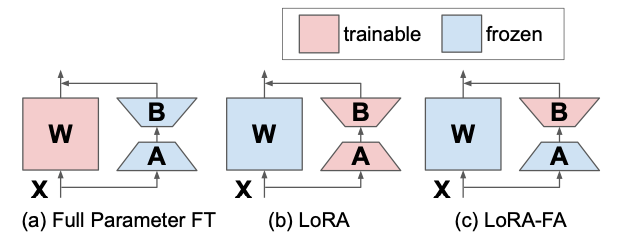
Another approach, LoRA-FA [4], which stands for LoRA with Frozen-A, is going in a similar direction as VeRA. In LoRA-FA, the matrix A is frozen after initialization and hence serves as a random projection. Instead of adding new vectors, matrix B is trained though, after being initialized with zeros (just as in the original LoRA). This halves the number of parameters while having comparable performance to normal LoRA.
LoRa-drop
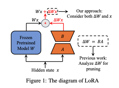
In the beginning, I explained, that you can add Lora matrices to any layer in the neural network. LoRA-drop [5] introduces an algorithm to decide which layers are worth to be enhanced by LoRA, and for which this is not worth the effort. Even if training LoRA adapters is much cheaper than finetuning the whole model, the more LoRA adapters you add, the more expensive is the training, still.
LoRA-drop consists of two steps. In the first step, you sample a subset of the data and train the LoRA adapters for a few iterations. Then you calculate the importance of each LoRA adapter as B*A*x, where A and B are the LoRA matrices, and x is the input. That is simply the output of the LoRA adapters that is added to the output of the frozen layer each. If this output is big, it changes the behavior of the frozen layer more drastically. If it is small, this indicates that the LoRA adapter has only little influence on the frozen layer and could as well be omitted.
Given that importance, you now select the LoRA layers that are most important. The are different ways of doing that. You can sum up the importance values until you reach a threshold, which is controlled by a hyperparameter, or you just take the top n LoRA layers with the highest importance for a fixed n. In any case, in the next step, you conduct the full training on the whole dataset (remember that you used a subset of data for the previous steps) but only on those layers that you just selected. The other layers are fixed to a shared set of parameters that won’t be changed anymore during training.
The algorithm of LoRA-drop hence allows to training a model with just a subset of the LoRA layers. The authors propose empirical evidence that indicates only marginal changes in accuracy, compared to training all LoRA layers, but at reduced computation time due to the smaller number of parameters that have to be trained.
AdaLoRA

There are alternative ways how to decide which LoRA parameters are more important than others. In this section, I will present AdaLoRA [6], which stands for Adaptive LoRa. What part of LoRA is adaptive here? It is the rank (i.e. the size) of the LoRA matrices. The main problem is the same as in the previous section: It may not be worth adding LoRA matrices A and B to each layer, but for some layers, the LoRA training may be more important (i.e. may lead to more change in the model’s behavior) than for others. To decide on that importance, the authors of AdaLoRA propose to consider the singular values of the LoRA matrices as indicators of their importance.
What is meant by that? First, we have to understand, that a matrix multiplication can also be seen as applying a function to a vector. When dealing with neural networks, this is quite obvious: Most of the time you use neural networks as functions, i.e. you give an input (say, a matrix of pixel values) and obtain a result (say, a classification of an image). Under the hood, this function application is powered by a sequence of matrix multiplications. Now, let’s say you want to reduce the number of parameters in such a matrix. That will change the function’s behavior, but you want it to change as little as possible. One way to do that is to compute the eigenvalues of the matrix, which tell you how much variance is captured by the rows of the matrix each. You may then decide to set some rows to zero, that capture only a small fraction of the variance, and hence don’t add much information to the function. This is the main idea of AdaLoRA since the aforementioned singular values are exactly the square roots of the eigenvalues. That is, based on the singular values, AdaLoRA decides which rows of which LoRA matrices are more important, and which can be omitted. This effectively shrinks the rank of some matrices, which have many rows that don’t contribute much. However, note an important difference to LoRA-drop from the previous section: In LoRA-drop, the adapter of a layer is selected to either be trained fully, or not trained at all. AdaLoRA can also decide to keep adaptors for some layers but with lower rank. That means, in the end, different adaptors can have different ranks (whereas in the original LoRA approach, all adaptors have the same rank).
There are some more details to the AdaLoRA approach, which I omitted for brevity. I want to mention two of them though: First, the AdaLoRA approach does not calculate the singular values explicitly all the time (as that would be very costly), but decomposes the weight matrices with a singular value decomposition. This decomposition is another way of representing the same information as in a single matrix, but it allows to get the singular values directly, without costly computation needed. Second, AdaLoRA does not decide on the singular values alone but also takes into account the sensitivity of the loss to certain parameters. If setting a parameter to zero has a large influence on the loss, this parameter is said to have high sensitivity. When deciding where to shrink the rank, the mean sensitivity of a row’s elements is taken into consideration in addition to the singular value.
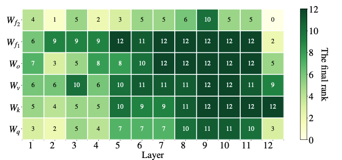
Empirical evidence for the value of the approach is given by comparing AdaLoRA with standard LoRA of the same rank budget. That is, both approaches have the same number of parameters in total, but these are distributed differently. In LoRA, all matrices have the same rank, while in AdaLoRA, some have a higher and some have a lower rank, which leads to the same number of parameters in the end. In many scenarios, AdaLoRA yields better scores than the standard LoRA approach, indicating a better distribution of trainable parameters on parts of the model, that are of particular importance for the given task. The following plot gives an example, of how AdaLoRA distributed the ranks for a given model. As we see, it gives higher ranks to the layers towards the end of the model, indicating that adapting these is more important.
DoRA
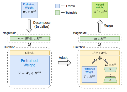
Another approach to modify LoRa to get better performance is Weight-Decomposed Low-Rank Adaption, or DoRA [7]. DoRA starts with the idea, that each matrix can be decomposed into the product of a magnitude and a direction. For a vector in 2D space, you can easily visualize that: A vector is nothing else than an arrow starting at the position of zero and ending at a certain point in the vector space. With the vector’s entries, you specify that point, e.g. by saying x=1 and y=1, if your space has two dimensions x and y. Alternatively, you could describe the very same point in a different way by specifying a magnitude and an angle (i.e. a direction), such as m=√2 and a=45°. That means that you start at point zero and move in the direction of 45° with an arrow length of √2. That will lead you to the same point (x=1,y=1).
This decomposition into magnitude and direction can also be done with matrices of higher order. The authors of DoRA apply this to the weight matrices that describe the updates within the training steps for a model trained with normal fine-tuning and a model trained with LoRA adapters. A comparison of these two techniques we see in the following plot:

We see two plots, one for a fine-tuned model (left) and one for a model trained with LoRA adapters (right). On the x-axis, we see the change in direction, on the y-axis we see the change in magnitude, and each scatter point in the plots belongs to one layer of the model. There is an important difference between the two ways of training. In the left plot, there is a small negative correlation between the update in direction and the update in magnitude, while in the right plot, there is a positive relationship, which is much stronger. You may wonder which is better, or whether this has any meaning at all. Remember, that the main idea of LoRA is to achieve the same performance as finetuning, but with fewer parameters. That means, ideally we want LoRA’s training to share as many properties with fine-tuning as possible, as long as this does not increase the costs. If the correlation between direction and magnitude is slightly negative in fine-tuning, this may be a desirable property for LoRA as well, if it is achievable. In other words, if the relationship between direction and magnitude is different in LoRA compared to full fine-tuning, this may be one of the reasons why LoRA sometimes performs less well than fine-tuning.
The authors of DoRA introduce a method to train magnitude and direction independently by separating the pretrained matrix W into a magnitude vector m of size 1 x d and a direction matrix V. The direction matrix V is then enhanced by B*A, as known from the standard LoRA approach, and m is trained as it is, which is feasible because it has just one dimension. While LoRA tends to change both magnitude and direction together (as indicated by the high positive correlation between these two), DoRA can more easily adjust the one without the other, or compensate changes in one with negative changes in the other. We can see the relationship between direction and magnitude is more like the one in finetuning:
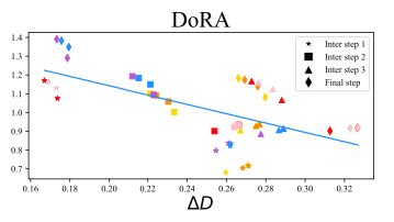
On several benchmarks, DoRA outperforms LoRA in accuracy. Decomposing the weight updates into magnitude and direction may allow DoRA to perform a training that is closer to the training done in fine-tuning, while still using the smaller parameters space introduced by LoRA.
Delta-LoRA
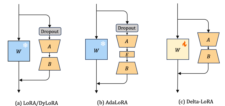
Delta-LoRA [8] introduces yet another idea to improve LoRA. This time, the pre-trained matrix W comes into play again. Remember that the main idea in LoRA is to not (!) tune the pre-trained matrix W, as that is too costly (and that would be normal fine-tuning). That is why LoRA introduced new smaller matrices A and B. However, those smaller matrices have less capability to learn the downstream task, which is why the performance of a LoRA-trained model is often lower than the performance of a fine-tuned model. Tuning W during training would be great, but how can we afford that?
The authors of Delta-LoRA propose to update the matrix W by the gradients of A*B, which is the difference between A*B in two consecutive time steps. This gradient is scaled with some hyperparameter λ, which controls, how big the influence of the new training on the pre-trained weights should be, and is then added to W (while α and r (the rank) are hyperparameters from the original LoRA setup):

That introduces more parameters to be trained at almost no computational overhead. We do not have to calculate the gradient for the whole matrix W, as we would within finetuning, but update it with a gradient we already got in the LoRA training anyway. The authors compared this method on a number of benchmarks using models like RoBERTA and GPT-2 and found a boost in performance over the standard LoRA approach.
Summary

We just saw a number of approaches, that vary the core idea of LoRA to reduce computation time or improve performance (or both). In the end, I will give a short summary of the different approaches:
- LoRA introduces low-rank matrices A and B that are trained, while the pre-trained weight matrix W is frozen.
- LoRA+ suggests having a much higher learning rate for B than for A.
- VeRA does not train A and B, but initializes them randomly and trains new vectors d and b on top.
- LoRA-FA only trains matrix B.
- LoRA-drop uses the output of B*A to determine, which layers are worth to be trained at all.
- AdaLoRA adapts the ranks of A and B in different layers dynamically, allowing for a higher rank in these layers, where more contribution to the model’s performance is expected.
- DoRA splits the LoRA adapter into two components of magnitude and direction and allows to train them more independently.
- Delta-LoRA changes the weights of W by the gradient of A*B.
The field of research on LoRA and related methods is very rich and vivid, with new contributions every other day. In this article, I wanted to explain the core ideas of some approaches. Naturally, that was only a selection of such, that is far away from being a complete review.
I hope that I have been able to share some knowledge with you and possibly inspire you to new ideas. LoRA and related methods are a field of research with great potential, as we saw. New breakthroughs in improving performance or computation time in training large language models can be expected soon, I suppose.
References and Further Reading
These are the papers on the concepts explained in this article:
- [1] LoRA: Hu, E. J., Shen, Y., Wallis, P., Allen-Zhu, Z., Li, Y., Wang, S., … & Chen, W. (2021). Lora: Low-rank adaptation of large language models. arXiv preprint arXiv:2106.09685.
- [2] LoRA+: Hayou, S., Ghosh, N., & Yu, B. (2024). LoRA+: Efficient Low Rank Adaptation of Large Models. arXiv preprint arXiv:2402.12354.
- [3] VeRA: Kopiczko, D. J., Blankevoort, T., & Asano, Y. M. (2023). Vera: Vector-based random matrix adaptation. arXiv preprint arXiv:2310.11454.
- [4]: LoRA-FA: Zhang, L., Zhang, L., Shi, S., Chu, X., & Li, B. (2023). Lora-fa: Memory-efficient low-rank adaptation for large language models fine-tuning. arXiv preprint arXiv:2308.03303.
- [5] LoRA-drop: Zhou, H., Lu, X., Xu, W., Zhu, C., & Zhao, T. (2024). LoRA-drop: Efficient LoRA Parameter Pruning based on Output Evaluation. arXiv preprint arXiv:2402.07721.
- [6] AdaLoRA: Zhang, Q., Chen, M., Bukharin, A., He, P., Cheng, Y., Chen, W., & Zhao, T. (2023). Adaptive budget allocation for parameter-efficient fine-tuning. arXiv preprint arXiv:2303.10512.
- [7] DoRA: Liu, S. Y., Wang, C. Y., Yin, H., Molchanov, P., Wang, Y. C. F., Cheng, K. T., & Chen, M. H. (2024). DoRA: Weight-Decomposed Low-Rank Adaptation. arXiv preprint arXiv:2402.09353.
- [8]: Delta-LoRA: Zi, B., Qi, X., Wang, L., Wang, J., Wong, K. F., & Zhang, L. (2023). Delta-lora: Fine-tuning high-rank parameters with the delta of low-rank matrices. arXiv preprint arXiv:2309.02411.
For some core ideas on random projection, as mentioned in the section on VeRA, this is one of the major contributions to the field:
For a more fine-grained explanation of LoRA and DoRA, I can recommend this article:
Like this article? Follow me to be notified of my future posts.
An Overview of the LoRA Family was originally published in Towards Data Science on Medium, where people are continuing the conversation by highlighting and responding to this story.
Originally appeared here:
An Overview of the LoRA Family