An Intuitive Introduction to Reinforcement Learning, Part I

Exploring popular reinforcement learning environments, in a beginner-friendly way

This is a guided series on introductory RL concepts using the environments from the OpenAI Gymnasium Python package. This first article will cover the high-level concepts necessary to understand and implement Q-learning to solve the “Frozen Lake” environment.

Happy learning ❤ !

Let’s explore reinforcement learning by comparing it to familiar examples from everyday life.

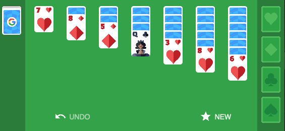
Card Game — Imagine playing a card game: When you first learn the game, the rules may be unclear. The cards you play might not be the most optimal and the strategies you use might be imperfect. As you play more and maybe win a few games, you learn what cards to play when and what strategies are better than others. Sometimes it’s better to bluff, but other times you should probably fold; saving a wild card for later use might be better than playing it immediately. Knowing what the optimal course of action is learned through a combination of experience and reward. Your experience comes from playing the game and you get rewarded when your strategies work well, perhaps leading to a victory or new high score.

Classical Conditioning — By ringing a bell before he fed a dog, Ivan Pavlov demonstrated the connection between external stimulus and a physiological response. The dog was conditioned to associate the sound of the bell with being fed and thus began to drool at the sound of the bell, even when no food was present. Though not strictly an example of reinforcement learning, through repeated experiences where the dog was rewarded with food at the sound of the bell, it still learned to associate the two together.

Feedback Control — An application of control theory found in engineering disciplines where a system’s behaviour can be adjusted by providing feedback to a controller. As a subset of feedback control, reinforcement learning requires feedback from our current environment to influence our actions. By providing feedback in the form of reward, we can incentivize our agent to pick the optimal course of action.

The Agent, State, and Environment

Reinforcement learning is a learning process built on the accumulation of past experiences coupled with quantifiable reward. In each example, we illustrate how our experiences can influence our actions and how reinforcing a positive association between reward and response could potentially be used to solve certain problems. If we can learn to associate reward with an optimal action, we could derive an algorithm that will select actions that yield the highest probable reward.

In reinforcement learning, the “learner” is called the agent. The agent interacts with our environment and, through its actions, learns what is considered “good” or “bad” based on the reward it receives.

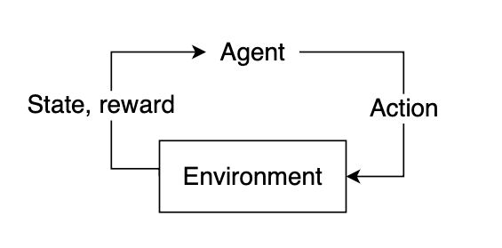
To select a course of action, our agent needs some information about our environment, given by the state. The state represents current information about the environment, such as position, velocity, time, etc. Our agent does not necessarily know the entirety of the current state. The information available to our agent at any given point in time is referred to as an observation, which contains some subset of information present in the state. Not all states are fully observable, and some states may require the agent to proceed knowing only a small fraction of what might actually be happening in the environment. Using the observation, our agent must infer what the best possible action might be based on learned experience and attempt to select the action that yields the highest expected reward.

After selecting an action, the environment will then respond by providing feedback in the form of an updated state and reward. This reward will help us determine if the action the agent took was optimal or not.

Markov Decision Processes (MDPs)

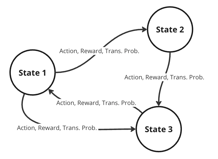
To better represent this problem, we might consider it as a Markov decision process (MDP). A MDP is a directed graph where each edge in the graph has a non-deterministic property. At each possible state in our graph, we have a set of actions we can choose from, with each action yielding some fixed reward and having some transitional probability of leading to some subsequent state. This means that the same actions are not guaranteed to lead to the same state every time since the transition from one state to another is not only dependent on the action, but the transitional probability as well.

Randomness in decision models is useful in practical RL, allowing for dynamic environments where the agent lacks full control. Turn-based games like chess require the opponent to make a move before you can go again. If the opponent plays randomly, the future state of the board is never guaranteed, and our agent must play while accounting for a multitude of different probable future states. When the agent takes some action, the next state is dependent on what the opponent plays and is therefore defined by a probability distribution across possible moves for the opponent.

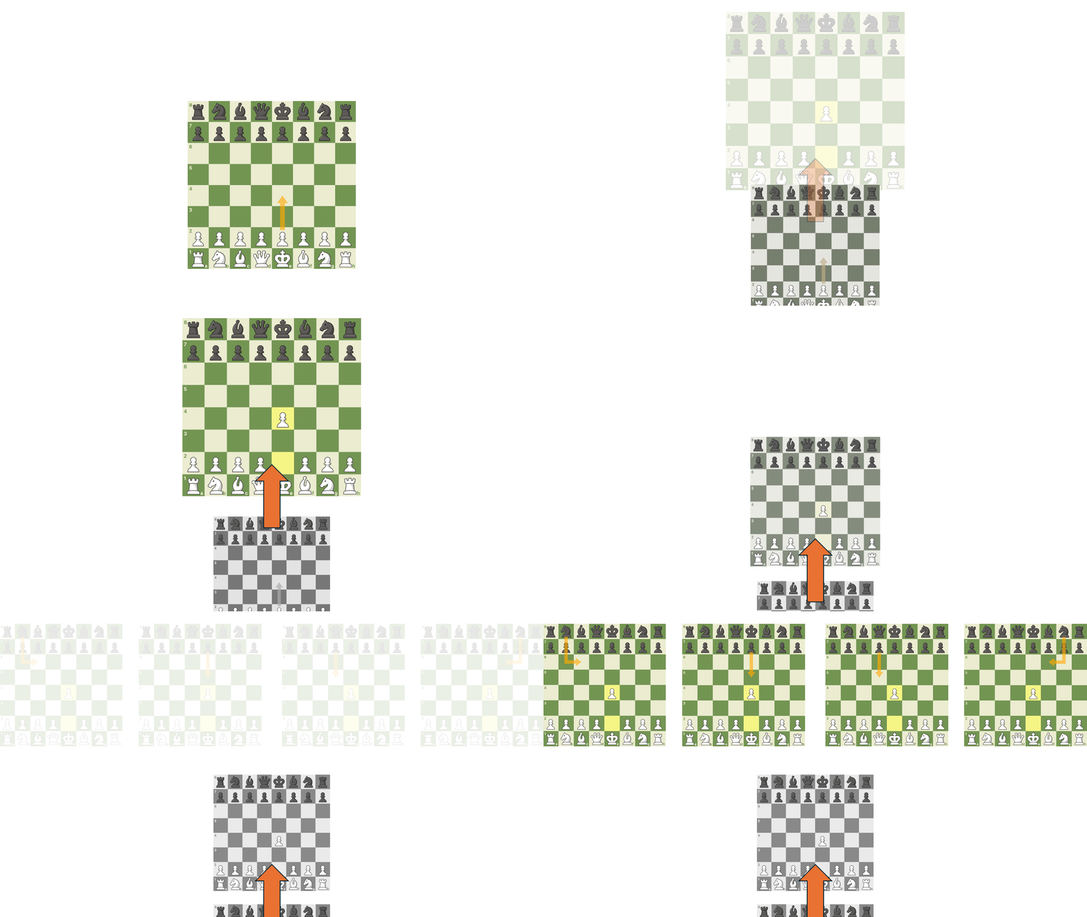
Our future state is therefore a function of both the probability of the agent selecting some action and the transitional probability of the opponent selecting some action. In general, we can assume that for any environment, the probability of our agent moving to some subsequent state from our current state is denoted by the joint probability of the agent selecting some action and the transitional probability of moving to that state.

Solving the MDP

To determine the optimal course of action, we want to provide our agent with lots of experience. Through repeated iterations of our environment, we aim to give the agent enough feedback that it can correctly choose the optimal action most, if not all, of the time. Recall our definition of reinforcement learning: a learning process built on the accumulation of past experiences coupled with quantifiable reward. After accumulating some experience, we want to use this experience to better select our future actions.

We can quantify our experiences by using them to predict the expected reward from future states. As we accumulate more experience, our predictions will become more accurate, converging to the true value after a certain number of iterations. For each reward that we receive, we can use that to update some information about our state, so the next time we encounter this state, we’ll have a better estimate of the reward that we might expect to receive.

Frozen Lake Problem

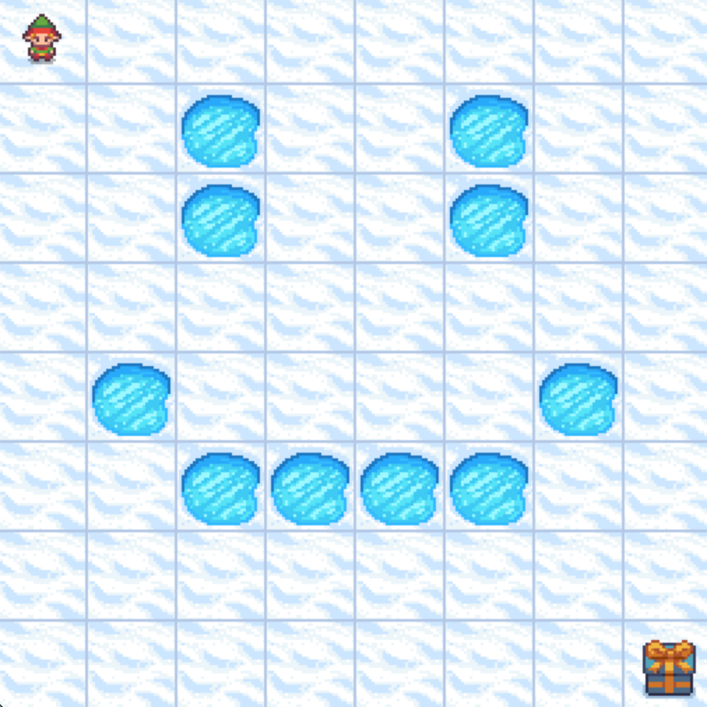
Let’s consider consider a simple environment where our agent is a small character trying to navigate across a frozen lake, represented as a 2D grid. It can move in four directions: down, up, left, or right. Our goal is to teach it to move from its start position at the top left to an end position located at the bottom right of the map while avoiding the holes in the ice. If our agent manages to successfully reach its destination, we’ll give it a reward of +1. For all other cases, the agent will receive a reward of 0, with the added condition that if it falls into a hole, the exploration will immediately terminate.

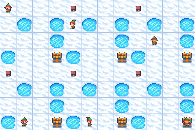
Each state can be denoted by its coordinate position in the grid, with the start position in the top left denoted as the origin (0, 0), and the bottom right ending position denoted as (3, 3).

The most generic solution would be to apply some pathfinding algorithm to find the shortest path to from top left to bottom right while avoiding holes in the ice. However, the probability that the agent can move from one state to another is not deterministic. Each time the agent tries to move, there is a 66% chance that it will “slip” and move to a random adjacent state. In other words, there is only a 33% chance of the action the agent chose actually occurring. A traditional pathfinding algorithm cannot handle the introduction of a transitional probability. Therefore, we need an algorithm that can handle stochastic environments, aka reinforcement learning.

This problem can easily be represented as a MDP, with each state in our grid having some transitional probability of moving to any adjacent state. To solve our MDP, we need to find the optimal course of action from any given state. Recall that if we can find a way to accurately predict the future rewards from each state, we can greedily choose the best possible path by selecting whichever state yields the highest expected reward. We will refer to this predicted reward as the state-value. More formally, the state-value will define the expected reward gained starting from some state plus an estimate of the expected rewards from all future states thereafter, assuming we act according to the same policy of choosing the highest expected reward. Initially, our agent will have no knowledge of what rewards to expect, so this estimate can be arbitrarily set to 0.

Let’s now define a way for us to select actions for our agent to take: We’ll begin with a table to store our predicted state-value estimates for each state, containing all zeros.

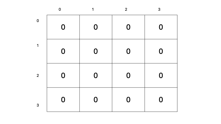
Our goal is to update these state-value estimates as we explore our environment. The more we traverse our environment, the more experience we will have, and the better our estimates will become. As our estimates improve, our state-values will become more accurate, and we will have a better representation of which states yield a higher reward, therefore allowing us to select actions based on which subsequent state has the highest state-value. This will surely work, right?

State-value vs. Action-value

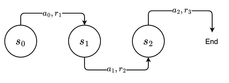
Nope, sorry. One immediate problem that you might notice is that simply selecting the next state based on the highest possible state-value isn’t going to work. When we look at the set of possible next states, we aren’t considering our current action—that is, the action that we will take from our current state to get to the next one. Based on our definition of reinforcement learning, the agent-environment feedback loop always consists of the agent taking some action and the environment responding with both state and reward. If we only look at the state-values for possible next states, we are considering the reward that we would receive starting from those states, which completely ignores the action (and consequent reward) we took to get there. Additionally, trying to select a maximum across the next possible states assumes we can even make it there in the first place. Sometimes, being a little more conservative will help us be more consistent in reaching the end goal; however, this is out of the scope of this article :(.

Instead of evaluating across the set of possible next states, we’d like to directly evaluate our available actions. If our previous state-value function consisted of the expected rewards starting from the next state, we’d like to update this function to now include the reward from taking an action from the current state to get to the next state, plus the expected rewards from there on. We’ll call this new estimate that includes our current action action-value.

We can now formally define our state-value and action-value functions based on rewards and transitional probability. We’ll use expected value to represent the relationship between reward and transitional probability. We’ll denote our state-value as V and our action-value as Q, based on standard conventions in RL literature.

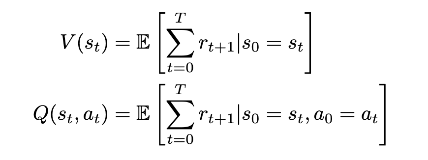
The state-value V of some state s[t] is the expected sum of rewards r[t] at each state starting from s[t] to some future state s[T]; the action-value Q of some state s[t] is the expected sum of rewards r[t] at each state starting by taking an action a[t] to some future state-action pair s[T], a[T].

This definition is actually not the most accurate or conventional, and we’ll improve on it later. However, it serves as a general idea of what we’re looking for: a quantitative measure of future rewards.

Our state-value function V is an estimate of the maximum sum of rewards r we would obtain starting from state s and continually moving to the states that give the highest reward. Our action-value function is an estimate of the maximum reward we would obtain by taking action from some starting state and continually choosing the optimal actions that yield the highest reward thereafter. In both cases, we choose the optimal action/state to move to based on the expected reward that we would receive and loop this process until we either fall into a hole or reach our goal.

Greedy Policy & Return

The method by which we choose our actions is called a policy. The policy is a function of state—given some state, it will output an action. In this case, since we want to select the next action based on maximizing the rewards, our policy can be defined as a function returning the action that yields the maximum action-value (Q-value) starting from our current state, or an argmax. Since we’re always selecting a maximum, we refer to this particular policy as greedy. We’ll denote our policy as a function of state s: π(s), formally defined as

To simplify our notation, we can also define a substitution for our sum of rewards, which we’ll call return, and a substitution for a sequence of states and actions, which we’ll call a trajectory. A trajectory, denoted by the Greek letter τ (tau), is denoted as

Since our environment is stochastic, it’s important to also consider the likelihood of such a trajectory occurring — low probability trajectories will reduce the expectation of reward. (Since our expected value consists of multiplying our reward by the transitional probability, trajectories that are less likely will have a lower expected reward compared to high probability ones.) The probability can be derived by considering the probability of each action and state happening incrementally: At any timestep in our MDP, we will select actions based on our policy, and the resulting state will be dependent on both the action we selected and the transitional probability. Without loss of generality, we’ll denote the transitional probability as a separate probability distribution, a function of both the current state and the attempted action. The conditional probability of some future state occurring is therefore defined as

And the probability of some action happening based on our policy is simply evaluated by passing our state into our policy function

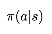
Our policy is currently deterministic, as it selects actions based on the highest expected action-value. In other words, actions that have a low action-value will never be selected, while actions with a high Q-value will always be selected. This results in a Bernoulli distribution across possible actions. This is very rarely beneficial, as we’ll see later.

Applying these expressions to our trajectory, we can define the probability of some trajectory occurring as

For clarity, here’s the original notation for a trajectory:

More concisely, we have

Defining both the trajectory and its probability allows us to substitute these expressions to simplify our definitions for both return and its expected value. The return (sum of rewards), which we’ll define as G based on conventions, can now be written as

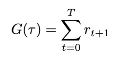
We can also define the expected return by introducing probability into the equation. Since we’ve already defined the probability of a trajectory, the expected return is therefore

We can now adjust the definition of our value functions to include the expected return

The main difference here is the addition of the subscript τ∼π indicating that our trajectory was sampled by following our policy (ie. our actions are selected based on the maximum Q-value). We’ve also removed the subscript t for clarity. Here’s the previous equation again for reference:

Discounted Return

So now we have a fairly well-defined expression for estimating return but before we can start iterating through our environment, there’s still some more things to consider. In our frozen lake, it’s fairly unlikely that our agent will continue to explore indefinitely. At some point, it will slip and fall into a hole, and the episode will terminate. However, in practice, RL environments might not have clearly defined endpoints, and training sessions might go on indefinitely. In these situations, given an indefinite amount of time, the expected return would approach infinity, and evaluating the state- and action-value would become impossible. Even in our case, setting a hard limit for computing return is oftentimes not beneficial, and if we set the limit too high, we could end up with pretty absurdly large numbers anyway. In these situations, it is important to ensure that our reward series will converge using a discount factor. This improves stability in the training process and ensures that our return will always be a finite value regardless of how far into the future we look. This type of discounted return is also referred to as infinite horizon discounted return.

To add discounting to our return equation, we’ll introduce a new variable γ (gamma) to represent the discount factor.

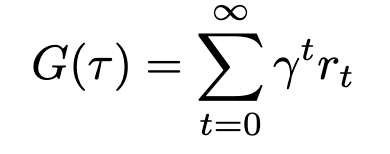
Gamma must always be less than 1, or our series will not converge. Expanding this expression makes this even more apparent

We can see that as time increases, gamma will be raised to a higher and higher power. As gamma is less than 1, raising it to a higher exponent will only make it smaller, thus exponentially decreasing the contribution of future rewards to the overall sum. We can substitute this updated definition of return back into our value functions, though nothing will visibly change since the variable is still the same.

Exploration vs. Exploitation

We mentioned earlier that always being greedy is not the best choice. Always selecting our actions based on the maximum Q-value will probably give us the highest chance of maximizing our reward, but that only holds when we have accurate estimates of those Q-values in the first place. To obtain accurate estimates, we need a lot of information, and we can only gain information by trying new things — that is, exploration.

When we select actions based on the highest estimated Q-value, we exploit our current knowledge base: we leverage our accumulated experiences in an attempt to maximize our reward. When we select actions based on any other metric, or even randomly, we explore alternative possibilities in an attempt to gain more useful information to update our Q-value estimates with. In reinforcement learning, we want to balance both exploration and exploitation. To properly exploit our knowledge, we need to have knowledge, and to gain knowledge, we need to explore.

Epsilon-Greedy Policy

We can balance exploration and exploitation by changing our policy from purely greedy to an epsilon-greedy one. An epsilon-greedy policy acts greedily most of the time with a probability of 1- ε, but has a probability of ε to act randomly. In other words, we’ll exploit our knowledge most of the time in an attempt to maximize reward, and we’ll explore occasionally to gain more knowledge. This is not the only way of balancing exploration and exploitation, but it is one of the simplest and easiest to implement.

Summary

Now the we’ve established a basis for understanding RL principles, we can move to discussing the actual algorithm — which will happen in the next article. For now, we’ll go over the high-level overview, combining all these concepts into a cohesive pseudo-code which we can delve into next time.

Q-Learning

The focus of this article was to establish the basis for understanding and implementing Q-learning. Q-learning consists of the following steps:

1. Initialize a tabular estimate of all action-values (Q-values), which we update as we iterate through our environment.
2. Select an action by sampling from our epsilon-greedy policy.
3. Collect the reward (if any) and update our estimate for our action-value.
4. Move to the next state, or terminate if we fall into a hole or reach the goal.
5. Loop steps 2–4 until our estimated Q-values converge.

Q-learning is an iterative process where we build estimates of action-value (and expected return), or “experience”, and use our experiences to identify which actions are the most rewarding for us to choose. These experiences are “learned” over many successive iterations of our environment and by leveraging them we will be able to consistently reach our goal, thus solving our MDP.

Glossary

• Environment — anything that cannot be arbitrarily changed by our agent, aka the world around it
• State — a particular condition of the environment
• Observation — some subset of information from the state
• Policy — a function that selects an action given a state
• Agent — our “learner” which acts according to a policy in our environment
• Reward — what our agent receives after performing certain actions
• Return — a sum of rewards across a series of actions
• Discounting — the process through which we ensure that our return does not reach infinity
• State-value — the expected return starting from a state and continuing to act according to some policy, forever
• Action-value — the expected return starting from a state and taking some action, and then continuing to act according to some policy, forever
• Trajectory — a series of states and actions
• Markov Decision Process (MDP) — the model we use to represent decision problems in RL aka a directed graph with non-deterministic edges
• Exploration — how we obtain more knowledge
• Exploitation — how we use our existing knowledge base to gain more reward
• Q-Learning — a RL algorithm where we iteratively update Q-values to obtain better estimates of which actions will yield higher expected return
• Reinforcement Learning — a learning process built on the accumulation of past experiences coupled with quantifiable reward

If you’ve read this far, consider leaving some feedback about the article — I’d appreciate it ❤.

References

[1] Gymnasium, Frozen Lake (n.d.), OpenAI Gymnasium Documentation.

[2] OpenAI, Spinning Up in Deep RL (n.d.), OpenAI.

[3] R. Sutton and A. Barto, Reinforcement Learning: An Introduction (2020), http://incompleteideas.net/book/RLbook2020.pdf

[4] Spiceworks, What is a Markov Decision Process? (n.d.), Spiceworks

[5] IBM, Reinforcement Learning (n.d.), IBM

An Intuitive Introduction to Reinforcement Learning, Part I was originally published in Towards Data Science on Medium, where people are continuing the conversation by highlighting and responding to this story.