An Introduction to Bayesian A/B Testing

Gain better insights from your data

A/B testing, also known as split testing, allows businesses to experiment with different versions of a webpage or marketing asset to determine which one performs better in terms of user engagement, click-through rates, and, most importantly, conversion rates.

Conversion rates — the percentage of visitors who complete a desired action, such as making a purchase or signing up for a newsletter — are often the key metrics that determine the success of online campaigns. By carefully testing variations of a webpage, businesses can make data-driven decisions that significantly improve these rates. Whether it’s tweaking the color of a call-to-action button, changing the headline, or rearranging the layout, A/B testing provides actionable insights that can transform the effectiveness of your online presence.

In this post, I will show how to do Bayesian A/B testing for looking at conversion rates. We will also look at a more complicated example where we will look at the differences in changes of customer behavior after an intervention. We will also look at the differences when comparing this approach to a frequentist approach and what the possible advantages or disadvantages are.

Comparing Conversion Rates

Let’s say we want to improve upon our e-commerce website. We do so by exposing two groups of customers to two versions of our website where we e.g. change a button. We then stop this experiment after having exposed a certain number of visitors to both these versions. After that, we get a binary array with a 1 indicating conversion and a 0 if there was no conversion.

We can summarize the data in a contingency table that shows us the (relative) frequencies.

contingency = np.array([[obsA.sum(), (1-obsA).sum()], [obsB.sum(), (1-obsB).sum()]])

In our case, we showed each variation to 100 customers. In the first variation, 5 (or 5%) converted, and in the second variation 3 converted.

Frequentist Setting

We will do a statistical test to measure if this result is significant or due to chance. In this case, we will use a Chi2 test which compares the observed frequencies to the ones that might be expected if there were no true differences between the two versions (the null hypothesis). For more information, one can look at this blog post that goes into more detail.

In this case, the p-value does not fall under the threshold for significance (e.g. 5%) and therefore we cannot reject the null hypothesis that the two variants differ in their effect on the conversion rate.

Now, there are some pitfalls when using the Chi2 test that can make the insights gained from it erroneous. Firstly, it is very sensitive to the sample size. With a large sample size even tiny differences will become significant whereas with a small sample size, the test may fail to detect differences. This is especially the case if the calculated expected frequencies for any of the fields are smaller than five. In this case, one has to use some other test. Additionally, the test does not provide information on the magnitude or practical significance of the difference. When conducting multiple A/B tests simultaneously, the probability of finding at least one significant result due to chance increases. The Chi2 test does not account for this multiple comparisons problem, which can lead to false positives if not properly controlled (e.g., through Bonferroni correction).

Another common pitfall occurs when interpreting the results of the Chi2 test (or any statistical test for that matter). The p-value gives us the probability of observing the data, given that the null hypothesis is true. It does not make a statement about the distribution of conversion rates or their difference. And this is a major problem. We cannot make statements such as “the probability that the conversion rate of variant B is 2% is X%” because for that we would need the probability distribution of the conversion rate (conditioned on the observed data).

These pitfalls highlight the importance of understanding the limitations of the Chi2 test and using it appropriately within its constraints. When applying this test, it is crucial to complement it with other statistical methods and contextual analysis to ensure accurate and meaningful conclusions.

Bayesian Setting

After looking at the frequentist way of dealing with A/B testing, let’s look at the Bayesian version. Here, we are modeling the data-generating process (and therefore the conversion rate) directly. That is, we are specifying a likelihood and a prior that could lead to the observed outcome. Think of this as specifying a ‘story’ for how the data could have been created.

In this case, I am using the Python package PyMC for modeling since it has a clear and concise syntax. Inside the ‘with’ statement, we specify distributions that we can combine and that give rise to a data-generating process.

with pm.Model() as ConversionModel:
    # priors
    pA = pm.Uniform('pA', 0, 1)
    pB = pm.Uniform('pB', 0, 1)
    
    delta = pm.Deterministic('delta', pA - pB)
    
    obsA = pm.Bernoulli('obsA', pA, observed=obsA)
    obsB = pm.Bernoulli('obsB', pB, observed=obsB)
    
    trace = pm.sample(2000)

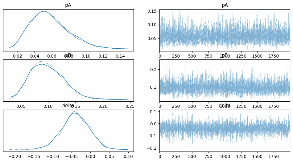
We have pA and pB which are the probabilities of conversion in groups A and B respectively. With pm.Uniform we specify our prior belief about these parameters. This is where we could encode prior knowledge. In our case, we are being neutral and allowing for any conversion rate between 0 and 1 to be equally likely.

PyMC then allows us to draw samples from the posterior distribution which is our updated belief about the parameters after seeing the data. We now obtain a full probability distribution for the conversion probabilities.

From these distributions, we can directly read quantities of interest such as credible intervals. This allows us to answer questions such as “What is the likelihood of a conversion rate between X% and Y%?”.

The Bayesian approach allows for much more flexibility as we will see later. Interpreting the results is also more straightforward and intuitive than in the frequentist setting.

Model Arbitrary Data-generating Processes

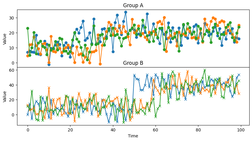
We will now look at a more complicated example of A/B testing. Let’s say we expose subjects to some intervention at the beginning of the observation period. This would be the A/B part where one group gets intervention A and the other intervention B. We then look at the interaction of the 2 groups with our platform in the next 100 days (maybe something like the number of logins). What we might see is the following.

We now want to know if these two groups show a meaningful difference in their response to the intervention. How would we solve this with a statistical test? Frankly, I don’t know. Someone would have to come up with a statistical test for exactly this scenario. The alternative is to again come back to a Bayesian setting, where we will first come up with a data-generating process. We will assume, that each individual is independent and its interactions with the platform are normally distributed. They have a switch point where they change their behavior. This switch point occurs only once but can happen at any given point in time. Before the switch point, we assume a mean interaction intensity of mu1 and after that an intensity of mu2. The syntax might look a bit complicated especially if you have never used PyMC before. In that case, I would recommend checking out their learning material.

with pm.Model(coords={
    'ind_id': ind_id,
}) as SwitchPointModel:

    sigma = pm.HalfCauchy("sigma", beta=2, dims="ind_id")

    # draw a switchpoint from a uniform distribution for each individual
    switchpoint = pm.DiscreteUniform("switchpoint", lower=0, upper=100, dims="ind_id")

    # priors for the two groups
    mu1 = pm.HalfNormal("mu1", sigma=10, dims="ind_id")
    mu2 = pm.HalfNormal("mu2", sigma=10, dims="ind_id")
    
    
    diff = pm.Deterministic("diff", mu1 - mu2)

    # create a deterministic variable for the 
    intercept = pm.math.switch(switchpoint < X.T, mu1, mu2)

    obsA = pm.Normal("y", mu=intercept, sigma=sigma, observed=obs)

    trace = pm.sample()

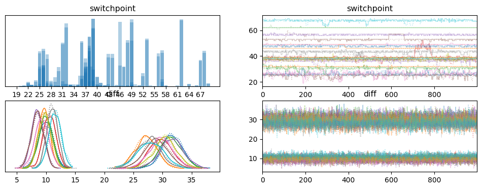
The model can then show us the distribution for the switch point location as well as the distribution of differences before and after the switch point.

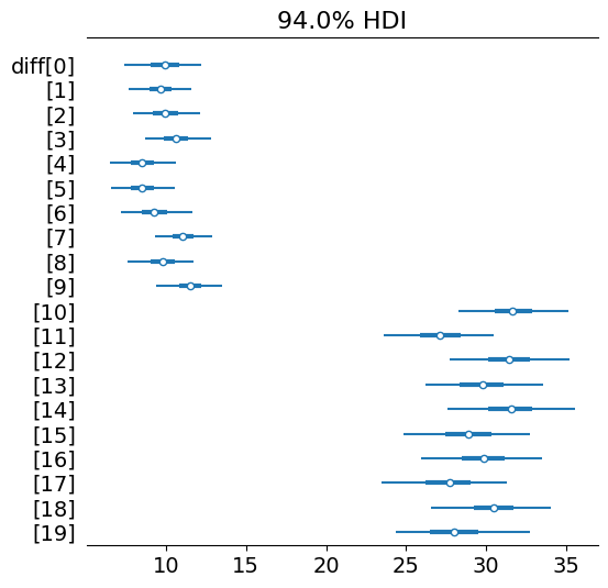
We can take a closer look at those differences with a forest plot.

We can nicely see how the differences between Group A (id 0 through 9) and Group B (10 through 19) are very much different where group B shows a much greater response to the intervention.

Conclusion

Bayesian Inference offers a lot of flexibility when it comes to modeling situations in which we do not have a lot of data and where we care about modeling uncertainty. Additionally, we have to make our assumptions explicit and think about them. In more simple scenarios, frequentist statistical tests are often simpler to use but one has to be aware of the assumptions that come along with them.

All code used in this article can be found on my GitHub. Unless otherwise stated, all images are created by the author.

An Introduction to Bayesian A/B Testing was originally published in Towards Data Science on Medium, where people are continuing the conversation by highlighting and responding to this story.