Advanced Retriever Techniques to Improve Your RAGs

Master Advanced Information Retrieval: Cutting-edge Techniques to Optimize the Selection of Relevant Documents with Langchain to Create Excellent RAGs

Content Table

· Introduction
· Vectore Store Creation
· Method: Naive Retriever
· Method: Parent Document Retriever
· Method: Self Query Retriever
∘ Query Constructor
∘ Query Translater
· Method: Contextual Compression Retriever (Reranking)
· Conclusion

Introduction

Let’s briefly remember what the 3 acronyms that make up the word RAG mean:

• Retrieval: The main objective of a RAG is to collect the most relevant documents/chunks regarding the query.
• Augmented: Create a well-structured prompt so that when the call is made to the LLM, it knows perfectly what its purpose is, what the context is and how it should respond.
• Generation: This is where the LLM comes into play. When the model is given good context (provided by the “Retrieval” step) and has clear instructions (provided by the “Augmented” step), it will generate high-value responses for the user.

As we can see, the generation of the response to a user’s query (If we apply a RAG for the purpose of Q&A), depends directly on how well we have built the “Augmented” and especially the “Retrieval”.

In this article we are going to focus exclusively on the “Retrieval” part. In this important process of returning the most relevant documents, the concept of vector store appears.

To create these retrievals, we will use the Langchain library.

The vectore store is nothing more than a vector database, which stores documents in vector format. This vector representation comes from the use of transformers. I’m not saying something you don’t know at the moment.

It is clear that the more robust and complete this vector store is, the better retriever we can run. We already know that the creation of this database is an art in itself. Depending on the size of the chunks or the embedding model we use, our RAG will be better or worse.

I make a clarification here:

In this post we are NOT going to discuss how to create this vector store.
In this post we are going to discuss some of the techniques used to retrieve relevant documents.

Since a picture is worth a thousand words, I suggest you take a look at the following:

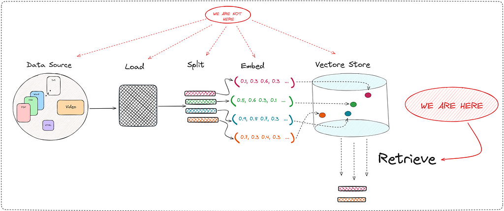
Therefore, I reiterate that in this post we are going to deeply study one of the many important steps in creating a good RAG tool. The “Retrieve” step is key since it directly improves the context that the LLM has when generating a response.

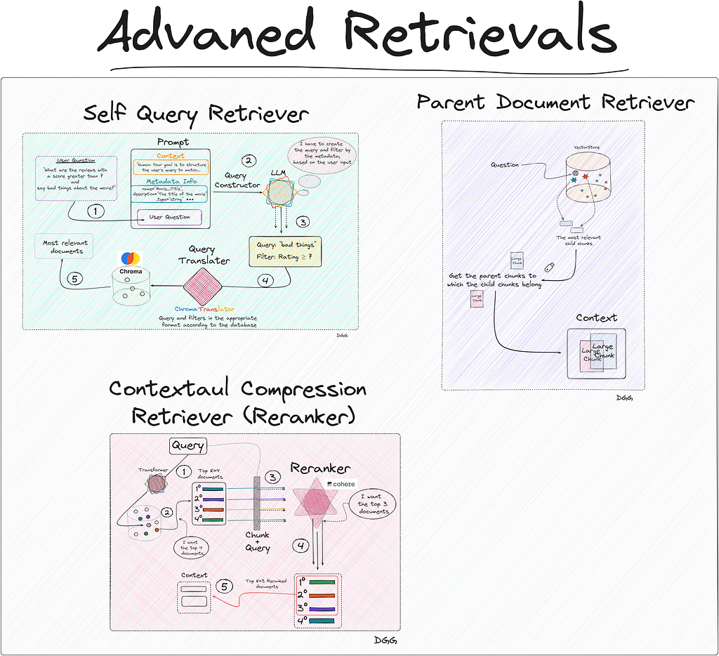
The methods we will study are:

• Naive Retriever
• Parent Document Retriever
• Self-Query Retriever
• Contextual Compression Retriever (Reranking)

You can find the project with the notebooks here. And you can also take a look at my github:

damiangilgonzalez1995 – Overview

Vectore Store Creation

To expose these methods, a practical use case will be carried out to improve the explanation. Therefore, we are going to create a RAG about reviews of the John Wick movies.

So that the reader can follow each step of this post, they can access the repository that I have created. In it you will find the code for each of the methods, in addition to the documents used to create the vector store. The jupyter notebook in charge of this task can be found in the git repository, and is the file called “0_create_vectore_db.ipynb”.

In relation to the data source of our RAG, there are 4 csv’s each corresponding to the reviews obtained for each of the films in the John Wick saga. The files contain the following information:

As you can see, the “Review” field will be the target of our retriever. The other fields being important to store as metadata:

• Movie_Title
• Review_Date
• Review_Title
• Review_Url
• Author
• Rating

To read and convert each row of our files into the “Document” format, we execute the following code:

from langchain_community.document_loaders.csv_loader import CSVLoader
from datetime import datetime, timedelta

documents = []

for i in range(1, 4):
  loader = CSVLoader(
    encoding="utf8",
    file_path=f"data/john_wick_{i}.csv",
    metadata_columns=["Review_Date", "Review_Title", "Review_Url", "Author", "Rating"]
  )

  movie_docs = loader.load()
  for doc in movie_docs:

    # We add metadate about the number of the movi
    doc.metadata["Movie_Title"] = f"John Wick {i}"

    # convert "Rating" to an `int`, if no rating is provided - None
    doc.metadata["Rating"] = int(doc.metadata["Rating"]) if doc.metadata["Rating"] else 5

  documents.extend(movie_docs)

We already have our documents in “Document” format:

print(documents[0])

Document(page_content=": 0nReview: The best way I can describe John Wick is to picture Taken but instead of Liam Neeson it's Keanu Reeves and instead of his daughter it's his dog. That's essentially the plot of the movie. John Wick (Reeves) is out to seek revenge on the people who took something he loved from him. It's a beautifully simple premise for an action movie - when action movies get convoluted, they get bad i.e. A Good Day to Die Hard. John Wick gives the viewers what they want: Awesome action, stylish stunts, kinetic chaos, and a relatable hero to tie it all together. John Wick succeeds in its simplicity.", metadata={'source': 'data/john_wick_1.csv', 'row': 0, 'Review_Date': '6 May 2015', 'Review_Title': ' Kinetic, concise, and stylish; John Wick kicks ***.n', 'Review_Url': '/review/rw3233896/?ref_=tt_urv', 'Author': 'lnvicta', 'Rating': 8, 'Movie_Title': 'John Wick 1', 'last_accessed_at': datetime.datetime(2024, 4, 8, 11, 49, 47, 92560)})

We only have to create a vector database (Vectore Store) locally. For this, I have used Chroma. Also keep in mind that it is necessary to use an embedding model, which will transform our documents into vector format for storage. Everything mentioned can be seen in the following piece of code:

from langchain_community.vectorstores import Chroma
from langchain_openai import OpenAIEmbeddings
import os
from dotenv import load_dotenv

load_dotenv()
os.environ["OPENAI_API_KEY"] = os.getenv('OPENAI_KEY')

embeddings = OpenAIEmbeddings(model="text-embedding-3-small")

db = Chroma.from_documents(documents=documents, embedding=embeddings, collection_name="doc_jonhWick", persist_directory="./jonhWick_db")

This will create a database on our premises called “JonhWick_db”. This will be the database that our RAG will use and from where our retriever will obtain the most relevant documents regarding the user’s queries.

Now is the time to present the different methods for creating a retriever.

Method: Naive Retriever

Code in 1_naive_retriever.ipynb file.

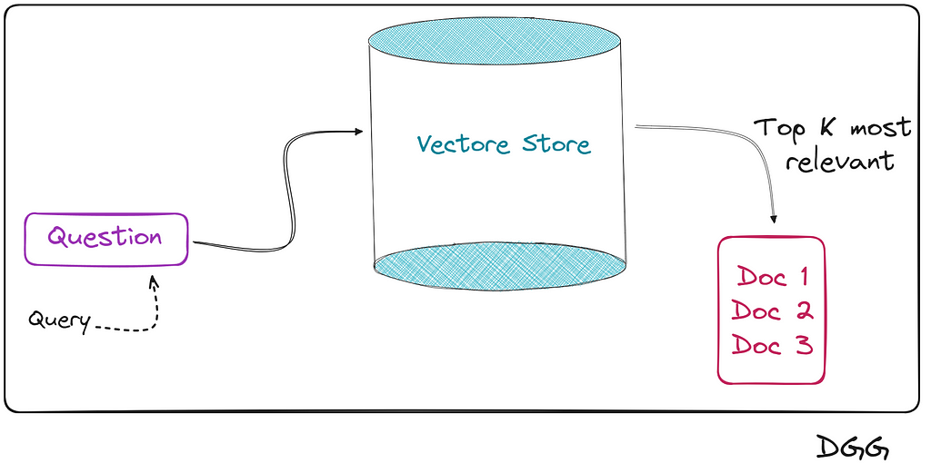
This method is the simplest, in fact its name indicates it. We use this adjective to identify this method for the simple reason that when entering the query into our database, we hope (naively) that it will return the most relevant documents/chunks.

Basically what happens is that we encode the user query with the same transformer with which we created the vector store. Once its vector representation is obtained, we calculate the similarity by calculating the cosine, the distance, etc.

And we collect the top K documents closest/similar to the query.

The flow of this type of retriever can be seen in the following image:

Keeping the scheme in mind, let’s see how all this looks in the code. We read the database:

from langchain_community.vectorstores import Chroma
from langchain_openai import OpenAIEmbeddings
import os
from dotenv import load_dotenv



load_dotenv()
os.environ["OPENAI_API_KEY"] = os.getenv('OPENAI_KEY')

embeddings = OpenAIEmbeddings(model="text-embedding-3-small")

vectordb= Chroma(persist_directory="./jonhWick_db", 
                  embedding_function=embeddings, 
                  collection_name="doc_jonhWick")pyth

And we create our retriever. We can configure the similarity calculation method, in addition to other parameters.

Retriever

# Specifying top k
naive_retriever = vectordb.as_retriever(search_kwargs={ "k" : 10})

# Similarity score threshold retrieval
# naive_retriever = db.as_retriever(search_kwargs={"score_threshold": 0.8}, search_type="similarity_score_threshold")

# Maximum marginal relevance retrieval
# naive_retriever = db.as_retriever(search_type="mmr")

Actually, we have already created our “Naive Retriever”, but to see how it works, we will create the complete RAG that we remember is composed of the following components:

• R (Retrieval): Done
• A (Augmented): Not yet
• G (Generation): Not yet

Augmented & Generation

from langchain_core.prompts import ChatPromptTemplate
from langchain_openai import ChatOpenAI

# Augmented
TEMPLATE = """
You are happy assistant. Use the context provided below to answer the question.

If you do not know the answer, or are unsure, say you don't know.

Query:
{question}

Context:
{context}
"""

rag_prompt = ChatPromptTemplate.from_template(TEMPLATE)


# Generation
chat_model = ChatOpenAI()

We already have the 3 components of our RAG. All that remains is to assemble them, and for this we will use the langchain chains to create a RAG.

I don’t know if you know the language created by langchain for creating chains in a more efficient way. This language is known as LCEL (LangChain Expression Language). If you are new to this way of creating chains in langchain, I leave you a very good tutorial here:

Finally, we create our RAG using Langchain’s own chain creation language (LCEL):

from langchain_core.runnables import RunnablePassthrough, RunnableParallel
from operator import itemgetter
from langchain_core.output_parsers import StrOutputParser

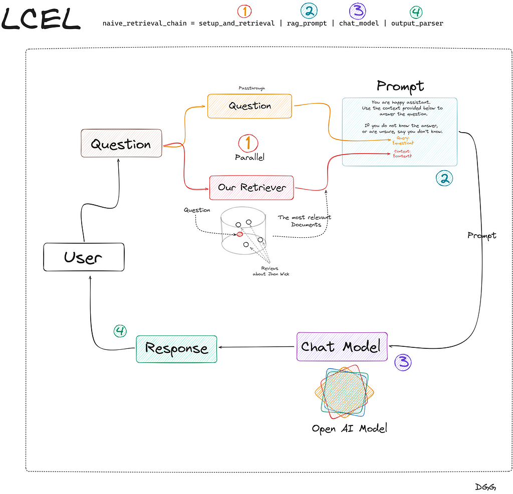
setup_and_retrieval = RunnableParallel({"question": RunnablePassthrough(), "context": naive_retriever })
output_parser = StrOutputParser()


naive_retrieval_chain = setup_and_retrieval 
                        | rag_prompt 
                        | chat_model 
                        | output_parser


naive_retrieval_chain.invoke( "Did people generally like John Wick?")


# response: 'Yes, people generally liked John Wick.'

This is the simplest way to create a chain for a RAG. In the Jupyter notebook you can find the same chain but more robust. Since I don’t want us to get lost on this topic now, I have only shown the simplest form. Also so that we understand what is happening in the code above, I have created this very clarifying diagram:

Great, we’re done creating our Naive RAG. Let’s move on to the next method.

Method: Parent Document Retriever

Code in 2_parent_document_retriever.ipynb file.

Imagine that we have created a RAG to recognize possible diseases by introducing some of their symptoms in the consultation. In the event that we have a Naive RAG, we may collect a series of possible diseases that only coincide in one or two symptoms, leaving our tool in a bit of a bad place.

This is an ideal case to use Parent Doc Retriever. And the type of technique consists of cutting large chunks (parent chunk) into even smaller pieces (child chunk). By having small chunks, the information they contain is more concentrated and therefore, its informative value is not diluted between paragraphs of text.

There is a small problem in all this:

• If we want to be precise in searching for the most relevant documents, we need to break our documents into small chunks.
• But it is also very important to provide good context to the LLM, which is achieved by providing larger chunks.

What has been said can be seen in the following image:

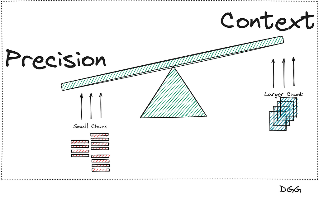
It seems that there is no way out of the problem, since when we increase the precision, the context is reduced, and vice versa. This is when this method appears that will solve our lives.

The main idea is to further chop the large chunks (Parent chunks/documents) into smaller chunks (Child Chunks/documents). Once this is done, perform the search for the most relevant top K documents with the child chunks, and return the parents chunks to which the top K child document belongs.

We already have the main idea, now let’s get it down to earth. The best way to explain it is step by step:

1. Obtain the documents and create the large chunks (Parent chunks)
2. Perform a split of each of the parent chunks for the growth of the child chunks.
3. Save the child chunks (Vector Representation) in the Vector Store.
4. Save the parent chunks in memory (We do not need to create their vector representation).

What has been said can be seen in the following image:

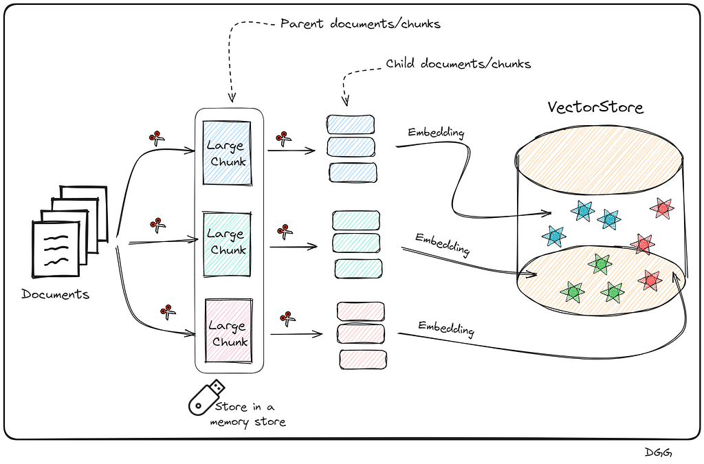
This may seem very complex to create, since we have to create a new database with the small chunks, save the parent chunks in memory. Additionally, know which parent chunk each child chunk belongs to. Thank goodness Langchain exists and the way to build it is super simple.

Surely you have come to the conclusion that it is necessary to create a new vector store for this method. Furthermore, in the case of reviews of the John Wick movies, such as the data source with CSV files, it is not necessary to perform the first split (parent chunks). This is because we can consider each row of our csv files to be a chunk in itself.

Overall, let’s visualize the following image that reflects how this method works:

Going to code it is represented as follows:

from langchain.retrievers import ParentDocumentRetriever
from langchain.storage import InMemoryStore
from langchain_text_splitters import RecursiveCharacterTextSplitter
from langchain_openai import OpenAIEmbeddings
from langchain_community.vectorstores import Chroma

# documents = Read csv files. Check jupyter notebook for more details

parent_docs = documents

# Embedding Model
embeddings = OpenAIEmbeddings(model="text-embedding-3-small")


# Splitters
child_splitter = RecursiveCharacterTextSplitter(chunk_size=200)
# We don't need a parent splitter because the data cames from CSV file, and each row is a parent doc.
# parent_splitter = RecursiveCharacterTextSplitter(chunk_size=800)

# Stores
store = InMemoryStore()
vectorstore = Chroma(embedding_function=embeddings, collection_name="fullDoc", persist_directory="./JohnWick_db_parentsRD")



parent_document_retriever = ParentDocumentRetriever(
    vectorstore=vectorstore,
    docstore=store,
    child_splitter=child_splitter,
    # parent_splitter =parent_splitter
)

Something intuitive about what happens here is that the number of chunks in the vector store (number of child chunks) should be much higher than the number of documents stored in memory (parent chunks). With the following code we can check it:

print(f"Number of parent chunks  is: {len(list(store.yield_keys()))}")

print(f"Number of child chunks is: {len(parent_document_retriever.vectorstore.get()['ids'])}")

'''
Number of parent chunks  is: 75
Number of child chunks is: 3701
'''

Great, we would already have our Parent Document Retriever, we just need to create our RAG based on this retriever and that would be it. It would be done exactly the same as in the previous method. I attach the code for creating the chain in langchain. To see more details, take a look at the jupyter notebook.

setup_and_retrieval = RunnableParallel({"question": RunnablePassthrough(), "context": parent_document_retriever })
output_parser = StrOutputParser()


parent_retrieval_chain = setup_and_retrieval | rag_prompt | chat_model | output_parser

Note that it is exactly the same as in the previous case, only with the small difference that in the “setup_and_retrieval” variable, we configure that we want to use our “parent_document_retriever”, instead of the “naive_retriever”.

Method: Self Query Retriever

Code in 3_self_query_retriever.ipynb file.

This is possibly one of the most optimal methods to improve the efficiency of our retriever.

Its main feature is that it is capable of performing searches in the vector store, applying filters based on the metadata.

We know that when we apply a “Naive retrieval”, we are calculating the similarity of all the chunks of the vector database with the query. The more chunks the vector store has, the more similarity calculations will have to be done. Now, imagine being able to do a prior filter based on the metadata, and after selecting the chunks that meet the conditions imposed in relation to the metadata, calculate similarities. This can drastically reduce computational and time cost.

Let’s look at a use case to fully understand when to apply this type of retreival.

Let’s imagine that we have stored in our vector database a large number of experiences and leisure offers (Ex: surf classes, zip line, gastronomic route, etc.). The description of the experience is what we have encoded, using our embedding model. Additionally, each offer has 3 key values or metadata: Date, price and place.

Let’s imagine that a user is looking for an experience of this style: An experience in nature, that is for the whole family and safe. Furthermore, the price must be less than $50 and the place is California.

Something is clear here

WE DO NOT WANT YOU TO RETURN US ACTIVITY/EXPERIENCES THAT DO NOT MEET THE PRICE OR PLACE THAT THE USER REQUESTS.

Therefore, it does not make sense to calculate similarities with chunks/experiences that do not comply with the metadata filter.

This case is ideal for applying Self Query Retriever. What this type of retriever allows us is to perform a first filter through the metadata, and then perform the similarity calculation between the chunks that meet the metadata requirements and the user input.

This technique can be summarized in two very specific steps:

• Query Constructor
• Query Translater

Query Constructor

The objective of the step called “Query Constructor” is to create the appropriate query and filters according to the user input.

Who is in charge of applying the corresponding filters and how do you know what they are?

For this we are going to use an LLM. This LLM will have to be able to decide which filters to apply and when. We will also have to explain beforehand what the metadata is and what each of them means. In short, the prompt must contain 3 key points:

• Context: Personality, how you should act, output format, etc.
• Metadata: Information about available metadata.
• Query: The user’s query/input/question.

The output generated by the LLM cannot be directly entered into the database. Therefore, the so-called “Query Translater” is needed.

Query Translater

This is a module in charge of translating the output of the LLM (Query Constructor) into the appropriate format to perform the query. Depending on the vector database you use, you will have to use one or the other. In my case I used Chroma db, therefore, I need a translator focused on this database. Luckily, Langchain has specific database translators for almost all of them.

As you may have already noticed, I am a big fan of diagrams. Let’s look at the following which provides quite a bit of clarity to the matter:

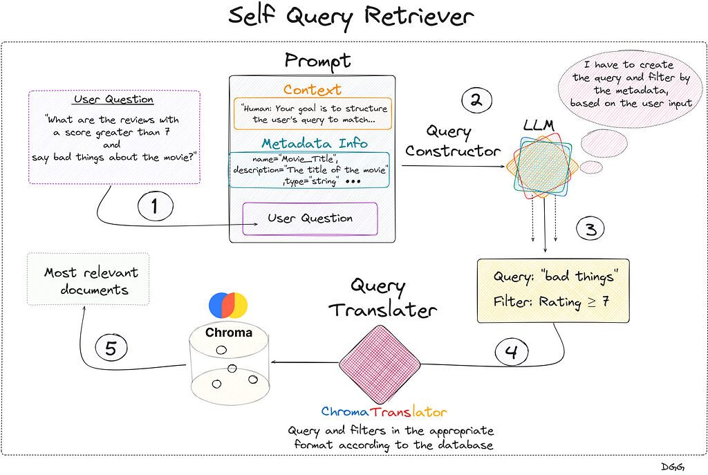
Regarding the previous image, we see that everything begins with the user’s query. We create the prompt that contains the 3 key fields and is introduced to the LLM that generates a response with two key fields: “Query” and “Filter”. This is fed into the query translator which translates these two fields into the correct format needed by Chroma DB. Performs the query and returns the most relevant documents based on the user’s initial question.

Something to emphasize is that the query entered by the user does not have to be the same as the one entered into the database. In the diagram shown, it can be seen that the LLM, taking into account the available metadata and the user’s question, detects that it can create a filter with the “Rating” metadata. It also creates a new query based on the user’s query.

Let’s look at all this in code. As I have explained, it is very important to provide the LLM with a detailed description of the metadata available in the vector store. This translates into the following piece of code:

from langchain.chains.query_constructor.base import AttributeInfo
from langchain.retrievers.self_query.base import SelfQueryRetriever
from langchain_openai import ChatOpenAI
from langchain.retrievers.self_query.chroma import ChromaTranslator



metadata_field_info = [
    AttributeInfo(
        name="Movie_Title",
        description="The title of the movie",
        type="string",
    ),
    AttributeInfo(
        name="Review_Date",
        description="The date of the review",
        type="string",
    ),
    AttributeInfo(
        name="Review_Title",
        description="The title of the review",
        type="string",
    ),
    AttributeInfo(
        name="Review_Url",
        description="The URL of the review",
        type="string",
    ),
    AttributeInfo(
        name="Author",
        description="The author of the review",
        type="string",
    ),
    AttributeInfo(
        name="Rating",
        description="A 1 to 10 rating for the movie",
        type="integer",
    )
]

To define our retrieval we must define the following points:

• The LLM to use
• The embedding model to be used
• The vector basis that is accessed
• A description of what information can be found in the
  documents of this vector base.
• The metadata description
• The Query translator you want to use

Let’s see what it looks like in code:

document_content_desription = "A review of the Jonh Wick movie."
embeddings = OpenAIEmbeddings(model="text-embedding-3-small")
chat_model = ChatOpenAI()

self_query_retriever = SelfQueryRetriever.from_llm(
    llm=ChatOpenAI(temperature=0),
    vectorstore =vectordb,
    document_contents = document_content_desription,
    metadata_field_info =metadata_field_info,
    verbose = True,
    structured_query_translator = ChromaTranslator()
)

Let’s see with a very clear example how we have greatly improved our RAG by using this type of retriever. First we use a naive retriever and then a self query retriever.

Question = "Make a summary of the reviews that talk about John Wick 3 and have a score higher than 7"
response = naive_retrieval_chain.invoke(Question)
print(response)

'''
I don't know the answer.
'''
------------------------------------------------------------------------

response = self_retrieval_chain.invoke(Question)
print(response)

'''
John Wick: Chapter 3 - Parabellum is quite literally 
about consequences, dealing with the fallout of John's...
'''

As we can see, there is a notable improvement.

Method: Contextual Compression Retriever (Reranking)

Code in 4_contextual_compression_retriever(reranking).ipynb file.

• Context Windows: The more documents we obtain from the vectore store, the more information the LLM will have to give a good answer.
• Recall: The more documents are retrieved from the vector store, the probability of obtaining irrelevant chunks is greater and therefore, the recall decreases (Not a good thing).

There seems to be no solution for this problem. When we increase one of the metrics, the other seems destined to decrease. Are we sure about that?

This is when this technique, compression retriever, is presented, focusing on the reranking technique. Let’s say that this technique consists of two very different steps:

• Step 1: Get a good amount of relevant docs based on the input/question. Normally we set the most relevant K.
• Step 2: Recalculate which of these documents are really relevant. discarding the other documents that are not really useful (Compression).

For the first step, what is known as Bi-Encoder is used, which is nothing more than what we usually use to make a basic RAG. Vectorize our documents. vectorize the query and calculate the similarity with any metric of our choice.

The second step is something different from what we are used to seeing. This recalculation/reranking is executed by the reranking model or cross-encoder.

These models expect two documents/texts as input, returning a similarity score between the pair.

If one of these two inputs is the query and the other is a chunk, we can calculate the similarity between the two.

These two methods can be displayed as follows:

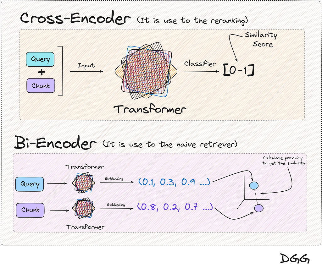
You will have realized that the two methods in the end provide the same result, a metric that reflects the similarity between two texts. And this is totally true, but there is a key feature:

The result returned by the cross encoder is much more reliable than with the Bi-encoder

Okay, it works better, then, because we don’t use it directly with all chunks, instead of just the top K chunks. Because it would be terribly expensive in time and money/computation. For this reason, we make a first filter of the chunks closest in similarity to the query, reducing the use of the reranking model to only K times.

A good question would be where to find the Cross-Encoder models? We are lucky that there are open source models that we can find in HuggingFace, but for the practical case of this post we are going to use the model made available by the company Cohere.

Cohere | The leading AI platform for enterprise

To better understand the architecture of this method, let’s look at a visual example.

The image shows the steps:

• 1º) We obtain the query, which we encode in its vector form with a transformer and we introduce it into the vector base.
• 2º) Collect the documents most similar to the query from our database. We can use any retriever method.
• 3º) Next we use the Cohere cross-encoder model. In the example in the image, this model will be used a total of 4 times. Remember that the input of this model will be the query and a document/chunk, to collect the similarity of these two texts.
• 4º) The 4 calls have been made to this model in the previous step and 4 new values (between 0 and 1) of the similarity between the query and each of the documents have been obtained. As can be seen, the chunk number 1 obtained in the previous steps, after the reranking, is now in 4th place.
• 5º) We add the first 3 chunks most relevant to the context.

Returning again to the computational cost and time, if the cross-encoders were applied directly, think that with each new query, the similarity of the query with each of the documents should be calculated. Something that is not optimal at all.

On the other hand, using Bi-Encoders, the vector representation of the documents is the same for each new query.

We then have a much superior method that is expensive to execute, and on the other hand, another method that works well but does not have a large computational cost with each new query. All this ends with the conclusion of unifying these two methods for a better RAG. And this is known as the Contextual Compression with reranking method.

Let’s move on to the code part. Let’s remember that this method uses a retreiver, which in our case will be a Naive Retriever:

naive_retriever = vectordb.as_retriever(search_kwargs={ "k" : 10})

Thanks to Langchain and its integration with Cohere, we only have to import the module that will execute the call to the Cohere cross-encoder model:

from langchain_cohere import CohereRerank

os.environ["COHERE_API_KEY"] = "YOUR API KEY FROM COHERE"

compressor = CohereRerank(top_n=3)

Finally, we create our Contextual Compression Retriever with Langchain:

from langchain.retrievers.contextual_compression import ContextualCompressionRetriever

compression_retriever = ContextualCompressionRetriever(
    base_compressor=compressor, 
    base_retriever=naive_retriever
)

As simple as that. Let’s see a comparison between a Naive Retriever and a Reranking Retriever:

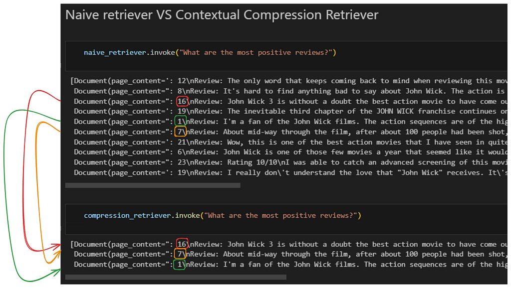
As we see, Naive returns us the top 10 chunks/documents. After performing the reranking and obtaining the 3 most relevant documents/chunks, there are noticeable changes. Notice how document number 16, which is in third position in relation to its relevance in the first retriever, becomes first position when performing the reranking.

Conclusion

We have seen that depending on the characteristics of the case where we want to apply a RAG, we will want to use one method or another. Furthermore, there may be the case in which one does not know which retriever method to use. For this, there are different libraries to evaluate your rags.

There are several tools for this purpose. Some of those options that I personally recommend are the combination of RAGAS and LangSmith.

Evaluating RAG pipelines with Ragas + LangSmith

I highly recommend following, learning and watching the videos of these people who are really what inspired me to make this article.

AI Makerspace

Thank you for reading!

If you find my work useful, you can subscribe to get an email every time that I publish a new article.

If you’d like, follow me on Linkedin!

Advanced Retriever Techniques to Improve Your RAGs was originally published in Towards Data Science on Medium, where people are continuing the conversation by highlighting and responding to this story.