A Whimsical Journey Through Wait Times

From Microwave Countdowns to Never-Ending Call Holds, with Python

Ever notice how microwave oven minutes march steadily toward zero, yet phone hold minutes stretch into eternity?

Consider this: barely a minute into microwaving your popcorn, you’re gathering bowls to be ready to serve. But a minute into a call hold? You’re wondering if you’ll ever speak to a human again. Fast forward 10 minutes, and you are enjoying your popcorn. But on the phone? The hold music has become the soundtrack for an endless purgatory.

And lurking in a twilight zone between waiting for popcorn and waiting on hold … your weekly lottery ticket. You wait for a win. Each week’s new ticket holds a fresh promise, a promise untouched by previous weekly disappointments.

To summarize, there appears to be three disparate types of waiting:

• “On Hold”-Type — The longer you’ve waited, the longer you expect to wait.
• “Popcorn”-Type — The longer you’ve waited, the less you expect to wait.
• “Lottery Win”-Type — Regardless of your wait so far, your expected wait remains the same.

Are these disparities in wait-times genuine, or a trick of the mind? We’ll answer this question in two parts.

• Part 1 — Analyzing Data
• Part 2 — Modeling Data

For each part, we’ll look at each type of waiting, alternating between detailed Python code and a discussion. If you are interested in Python, read the code sections. If you are only interested in learning about wait times, you may skip over the code.

Part 1: Analyzing Data

“On Hold”-Type Waits — The longer you’ve waited, the longer you expect to wait.

We’d like to start with data, but I don’t have data for “on hold” times. So, instead, how about the time between edits of a computer file? One place that I see such edit times is on Wikipedia.

Suppose I place you on a Wikipedia page. Can you look at just the time since the last edit and predict how long until the next edit?

Aside 1: No fair editing the page yourself.
Aside 2: Analogously, if I somehow place you “on hold” for some number of minutes (so far), can you predict how much longer until the call is re-connected?

For Wikipedia page edits, how might you express your prediction of the time until the next edit? You could try to predict the exact moment of the next edit, for example: “I predict this page will next be edited in exactly 5 days, 3 hours, 20 minutes” That, however, seems too specific, and you’d nearly always be wrong.

You could predict a range of times: “I predict this page will be next edited sometime between now and 100 years from now”. That would nearly always be right but is vague and uninteresting.

A more practical prediction takes the form of the “median next-edit time”. You might say: “I predict a 50% chance that this page will be edited within the next 5 days, 3 hours, 20 minutes.” I, your adversary, would then pick “before” or “after”. Suppose I think the real median next-edit time is 3 days. I would then pick “before”. We then wait up to 5 days, 3 hours, 20 minutes. If anyone (again, other than us) edits the page in that time, I get a point; otherwise, you get a point. With this scoring system, if you’re a better predictor than I, you should earn more points.

Let’s next dive into Python and see how we might make such predictions:

“On Hold”-Type Waits — Python

Consider the Wikipedia article about the artist Marie Cochran. We can look at the article’s revision history:

To gather such data from various Wikipedia articles, I wrote a little Python script that:

• Picks a random English-language Wikipedia page via https://en.wikipedia.org/wiki/Special:Random.
• Goes to that page’s revision history, for example, https://en.wikipedia.org/w/index.php?title=Marie_Cochran&action=history.
• Pulls out the date and times of (up to the) last 50 edits. Times are to the resolution of a minute.
• Creates lines made up of the article title, an edit time, and the time of the script’s run. All times use the UTC time zone. Tabs separate columns.
• Appends the lines to a file.

Aside: This approach brings up several issues. First, in what sense Special:Random random? I don’t know. For the purpose of this demonstration, it seems random enough. Why up-to-the-last 50 edits? Why not all the edits? Why not just the most recent edit? I don’t have a good reason beyond “up-to-the-last 50” is the default and works well enough for this article. Finally, why script against the regular Wikipedia server when we could instead retrieve the full edit history for all articles from https://dumps.wikimedia.org? Because we only need a sample. Also, writing this script was easy, but writing a program to process the full data would be hard. Sadly, I will not share the easy script because I don’t want to enable uncontrolled bots hitting the Wikipedia site. Happily, I am sharing on GitHub all the data I collected. You may use it as you wish.

Here is a fragment of the edit time data:

Marie_Cochran 01:20, 8 January 2024 01:16, 08 February 2024
Marie_Cochran 01:10, 27 September 2023 01:16, 08 February 2024
Marie_Cochran 00:59, 12 September 2023 01:16, 08 February 2024
Marie_Cochran 11:43, 2 November 2022 01:16, 08 February 2024
...
Marie_Cochran 19:20, 10 March 2018 01:16, 08 February 2024
Peter_Tennant 15:03, 29 July 2023 01:16, 08 February 2024
Peter_Tennant 21:39, 15 April 2022 01:16, 08 February 2024
...

Let’s read this into a Pandas dataframe and compute Time Delta, the wait times between edits:

import pandas as pd

# Read the data
wiki_df = pd.read_csv("edit_history.txt", sep='t', header=None, names=["Title", "Edit DateTime", "Probe DateTime"], usecols=["Title", "Edit DateTime"])
wiki_df['Edit DateTime'] = pd.to_datetime(wiki_df['Edit DateTime']) # text to datetime

# Sort the DataFrame by 'Title' and 'Edit DateTime' to ensure the deltas are calculated correctly
wiki_df.sort_values(by=['Title', 'Edit DateTime'], inplace=True)

# Calculate the time deltas for consecutive edits within the same title
wiki_df['Time Delta'] = wiki_df.groupby('Title')['Edit DateTime'].diff()
wiki_df.head()

The resulting Pandas dataframe starts with the alphabetically-first article (among those sampled). That article tells readers about Öndör Gongor, a very tall person from Mongolia:

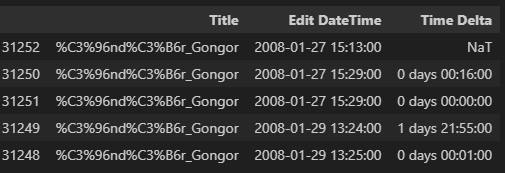
Within that article’s last 50 edits, we first see an edit on January 27th, 2008, at 3:13 PM (UTC). We next see an edit 16 minutes later. The edit after that occurs within a minute (the limit of the data’s resolution) and so shows 0 days 00:00:00.

Continuing our processing, let’s drop the NaT (not-a-time) rows that appear at the start of each article. We’ll also sort by the wait times and reset Panda’s index:

# Remove rows with not-a-time (NaT) values in the 'Time Delta' column
wiki_df.dropna(subset=['Time Delta'], inplace=True)
# Sort by time delta and reset the index
wiki_df.sort_values(by='Time Delta', inplace=True)
wiki_df.reset_index(drop=True, inplace=True)
display(wiki_df)
wiki_df['Time Delta'].describe()

This produces a dataframe that start and ends like this:

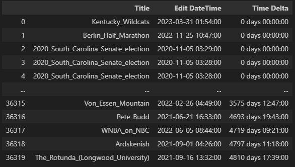
with this statistical summary:

count                          36320
mean      92 days 13:46:11.116189427
std      195 days 11:36:52.016155110
min                  0 days 00:00:00
25%                  0 days 00:27:00
50%                 15 days 05:41:00
75%                100 days 21:45:45
max               4810 days 17:39:00

We see that the sampled wait times vary from 0 days 00:00:00 (so, less than a minute) to over 13 years. (The 13 year edit wait was for an article about a building at a Virginia university.) One quarter of the edits happen within 27 minutes of a previous edit. The median time between edits is just over 15 days.

Before we go farther, I want to improve the display of wait times with a little function:

def seconds_to_text(seconds):
    seconds = round(seconds)
    result = []
    for unit_name, unit_seconds in [('y', 86400 * 365.25),('d', 86400),('h', 3600),('m', 60),('s', 1)]:
        if seconds >= unit_seconds:
            unit_value, seconds = divmod(seconds, unit_seconds)
            result.append(f"{int(unit_value)}{unit_name}")
    return ' '.join(result) if result else "<1s"

seconds_to_text(100)

The seconds_to_text function displays 100 seconds as ‘1m 40s’.

With this we can construct a “wait wait” table for the Wikipedia data. Given the wait so far for the next edit on an article, the table tells our median additional wait. (Recall that “median” means that half the time, we expect to wait less than this time for an edit. The other half of the time, we expect to wait more than this time.)

import numpy as np

def wait_wait_table(df, wait_ticks):
    sorted_time_deltas_seconds = df['Time Delta'].dt.total_seconds()
    results = []
    for wait_tick in wait_ticks:
        greater_or_equal_values = sorted_time_deltas_seconds[sorted_time_deltas_seconds >= wait_tick]
        median_wait = np.median(greater_or_equal_values)
        additional_wait = median_wait - wait_tick
        results.append({"Wait So Far": seconds_to_text(wait_tick), "Median Additional Wait": seconds_to_text(additional_wait)})
    return pd.DataFrame(results)

wiki_wait_ticks = [0, 60, 60*5, 60*15, 3600, 3600*4, 86400, 86400 * 7,86400 * 30, 86400 * 100, 86400 * 365.25, 86400 * 365.25 * 5, 86400 * 365.25 * 10]
wiki_wait_tick_labels = [seconds_to_text(wait_tick) for wait_tick in wiki_wait_ticks]
wait_wait_table(wiki_df, wiki_wait_ticks).style.hide(axis="index")

We’ll discuss the output of this table next.

“On Hold”-Type Waits — Discussion

The preceding Python code produces this table. Call it a “wait-wait” table.

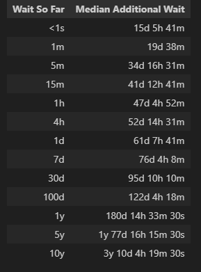
The table says that if we haven’t waited at all (in other words, someone just edited the page), we can anticipate the next edit in just over 15 days. However, if after a minute, no one has edited the article again, we can anticipate a wait of 19 days. Thus, waiting one minute leads to almost 4 days more of additional expected waiting. If, after one hour, no one has edited the article, our anticipated additional wait more-than-doubles to 47 days.

Aside: When I use the term ‘anticipate’ in this context, I’m referring to the median waiting time derived from our historical data. In other words, based on past trends, we bet that half of the very next edits will occur sooner than this time frame, and half will occur later.

One way to think about this phenomenon: When we start our wait for the next edit, we don’t know what kind of page we are on. Is this an article about a hot pop-culture topic such as Taylor Swift? Or is this an article about a niche, slow-moving topic such as The Rotunda, a building at a 5000-student university. With every minute that passes without an edit, the probabilities shift from this being a Taylor-Swift-like article and toward a The-Rotunda-like article.

Likewise, when we call customer service and are put on hold — at the start we don’t know what kind of customer service we are waiting on. With every passing minute, however, we learn that we are likely waiting for poor, slow customer service. Our anticipated additional wait, thus, grows.

Up to this point, we have used the data directly. We can also try to model the data with a probability distribution. Before we move to modeling, however, let’s look at our other two examples: microwaving popcorn and waiting for a lotto win.

“Popcorn”-type Waits — The longer you’ve waited, the less you expect to wait.

Let’s apply the techniques from waiting for Wikipedia edits to waiting for microwave popcorn. Rather than collecting real data (as delicious as that might be), I’m content to simulate data. We’ll use a random number generator. We assume that the time to cook, perhaps based on a sensor, is 5 minutes plus or minus 15 seconds.

“Popcorn”-type Waits — Python

Specifically in Python:

seed = 0
rng = np.random.default_rng(seed)
sorted_popcorn_time_deltas = np.sort(rng.normal(5*60, 15, 30_000))
popcorn_df = pd.DataFrame(pd.to_timedelta(sorted_popcorn_time_deltas,unit="s"), columns=["Time Delta"])
print(popcorn_df.describe())

Which produces a Panda dataframe with this statistical summary:

                      Time Delta
count                      30000
mean   0 days 00:05:00.060355606
std    0 days 00:00:14.956424467
min    0 days 00:03:52.588244397
25%    0 days 00:04:50.011437922
50%    0 days 00:04:59.971380399
75%    0 days 00:05:10.239357827
max    0 days 00:05:59.183245298

As expected, when generating data from this normal distribution, the mean is 5 minutes, and the standard deviation is about 15 seconds. Our simulated waits range from 3 minutes 52 seconds to 6 minutes.

We can now generate a “wait-wait” table:

wait_wait_table(popcorn_df, [0, 10, 30, 60, 2*60, 3*60, 4*60, 5*60]).style.hide(axis="index")

“Popcorn”-type Waits — Discussion

Our “wait-wait” table for popcorn looks like this:

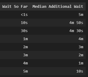
Our table says that at the beginning, we expect a 5-minute wait. After we wait for 10 seconds, our additional expected wait falls exactly 10 seconds (to 4 minutes 50 seconds). After we wait one minute, our additional wait falls to 4 minutes and so on. At 5 minutes, the anticipated additional wait continues to go down (but not to zero).

In a later section, we’ll see how to model this data. For now, let’s look next at waiting for a lottery win.

“Lottery Win”-Style Waits — Regardless of your wait so far, your expected wait remains the same.

For lottery data, I’m again comfortable creating simulated data. The Washington State Lotto offers odds of 1 to 27.1 for a win. (The most common win, pays $3 for a $1 bet.) Let’s play the lotto for 1 million weeks (about 19,000 years) and collect data on our waits between wins.

“Lottery Win”-Style Waits — Python

We simulate 1 million weeks of lotto play:

seed = 0
rng = np.random.default_rng(seed)
last_week_won = None
lotto_waits = []
for week in range(1_000_000):
    if rng.uniform(high=27.1) < 1.0:
        if last_week_won is not None:
            lotto_waits.append(week - last_week_won)
        last_week_won = week
sorted_lotto_time_deltas = np.sort(np.array(lotto_waits) * 7 * 24 * 60 * 60)
lotto_df = pd.DataFrame(pd.to_timedelta(sorted_lotto_time_deltas,unit="s"), columns=["Time Delta"])
print(lotto_df.describe())

                        Time Delta
count                        36773
mean   190 days 08:21:00.141951976
std    185 days 22:42:41.462765808
min                7 days 00:00:00
25%               56 days 00:00:00
50%              133 days 00:00:00
75%              259 days 00:00:00
max             2429 days 00:00:00

Our shortest possible interval between wins is 7 days. Our longest simulated dry spell is over 6 years. Our median wait is 133 days.

We generate the “wait-wait” table with:

lotto_days = [0, 7, 7.00001,  2*7, 4*7, 183, 365.25, 2*365.25, 5*365.25]
lotto_waits = [day * 24 * 60 * 60 for day in lotto_days]
wait_wait_table(lotto_df, lotto_waits).style.hide(axis="index")

“Lottery Win”-Style Waits — Discussion

Here is the “wait-wait” table:

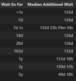
The table shows that the lotto doesn’t care how long we’ve waited for a win. Whether we just won (Wait So Far < 1s) or haven’t won for a year, our anticipated additional wait until our next win is almost always between 126 days and 133 days.

Three entries on the table might seem strange. What do you think is going on at 7d and 7d 1s? Why does the additional wait jump, almost instantly from 126 days to about 133 days? The answer is at the moment of the weekly drawing, the minimum wait for a win shifts from 0 days to 7 days. And what about 5y? Is this showing that if we wait 5 years, we can anticipate a win in just 50 days, much less than the usual 133 days? Sadly, no. Rather it shows the limitation of our data. In the data, we only see 5-year waits three times:

lotto_df[lotto_df["Time Delta"] > pd.to_timedelta(24*60*60 * 365.25 * 5, unit="s")]

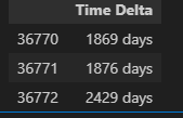
Three values lead to a noisy estimate of the median.

To summarize what we’ve seen so far in real and simulated data:

• Wikipedia Edits —The longer you’ve waited, the longer you expect to wait
• Popcorn — The longer you’ve waited, the less you expect to wait
• Lottery Wins— Regardless of your wait so far, your expected wait remains the same

In the next section, we’ll look at the hows and (importantly) the whys of modeling. We’ll start with our lotto data.

Part 2: Modeling Data

In this part, we’ll try to find simple expressions for wait-time predictions. Such simplicity is not needed for predictions. What we’ve created so far, called an empirical distribution, works fine. A simpler expression can, however, be more convenient. Also, it may make comparisons between different types of waits easier to understand.

We will proceed by looking at our three examples starting with the simplest (Lottery Wins) to the most complex (Wikipedia Edits). As before, I’ll alternate between Python code (that you can skip over) and discussion.

We’ll start by adding a cumulative distribution column to our three wait-time dataframes. Recall that we previously sorted the dataframes by Time Delta.

wiki_df['CDF'] = wiki_df['Time Delta'].rank(pct=True)
popcorn_df['CDF'] = popcorn_df['Time Delta'].rank(pct=True)
lotto_df['CDF'] = lotto_df['Time Delta'].rank(pct=True)
wiki_df

The column labeled CDF, for cumulative distribution function, contains values near 0.0 for the shortest wait times and a value of 1.0 for the longest wait time. In other words, it is the rank of each row expressed as a fraction. The Wikipedia dataframe now looks like:

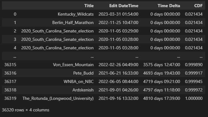
We can now plot CDF (y-axis) vs. the wait time Time Delta (x-axis). Here is some plotting code in Python:

import matplotlib.pyplot as plt

def wait_cdf(title, sorted_df, wait_ticks, dist=None, dist_label=None, left=None, right=None, xscale='linear'):
    wait_seconds = sorted_df['Time Delta'].dt.total_seconds() # x values
    cdf = sorted_df['CDF'] # y values

    left = left or wait_seconds.min()
    right = right or wait_seconds.max()

    plt.figure(figsize=(10, 6))
    plt.title(title + ' Cumulative Distribution Function (CDF)')
    plt.plot(wait_seconds, cdf, marker='.', linestyle=" ", label='Empirical CDF')

    if dist is not None:
        dist_x = np.logspace(np.log10(left), np.log10(right), 100) if xscale == 'log' else np.linspace(left, right, 100)
        dist_y = dist.cdf(dist_x)
        plt.plot(dist_x, dist_y, label = dist_label)

    plt.xlabel('Wait')
    plt.ylabel('CDF')
    plt.xscale(xscale)
    plt.xticks(wait_ticks, [seconds_to_text(wait_tick) for wait_tick in wait_ticks], rotation=45)
    plt.xlim(left=left, right=right)
    plt.grid(True, which="both", ls="--")
    plt.legend(loc='upper left')
    plt.show()

wait_cdf("Lottery Wins", lotto_df, wiki_wait_ticks, xscale='log')

Here is the CDF plot of Lottery Wins with wait time on a log scale:

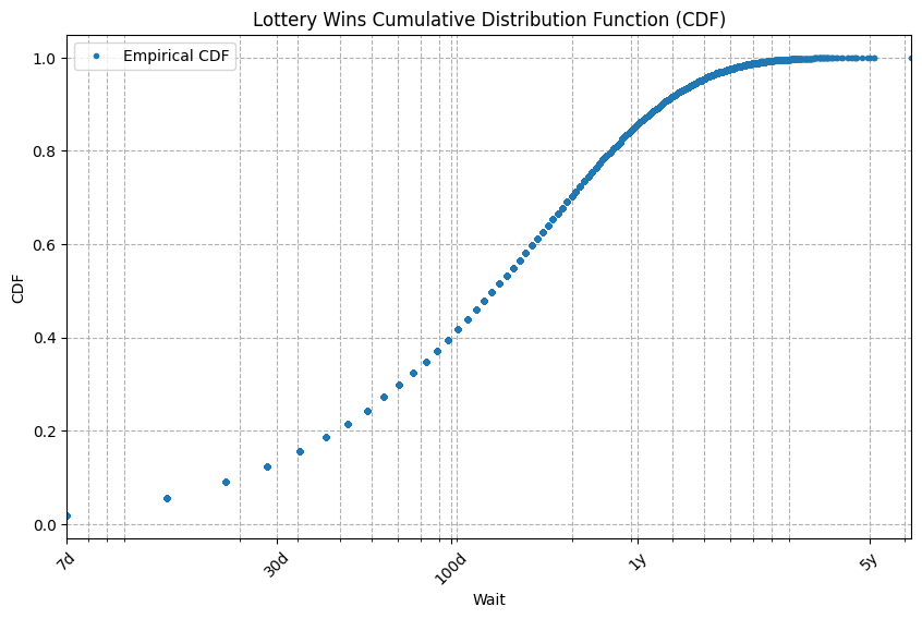
The curve looks simple so let’s try to fit a simple curve to it. The obvious candidate curve is the exponential distribution. It’s the simplest common function related to wait times.

Python’s scipy.stats package makes it easy to fit an exponential curve to our data and to represent the resulting curve as a Python object, here named lotto_expon_dist.

from scipy.stats import expon

_, lotto_e_scale = expon.fit(lotto_df['Time Delta'].dt.total_seconds(), floc=0)
lotto_expon_dist = expon(scale=lotto_e_scale)
print(f"Lottery wins exponential median is {seconds_to_text(lotto_expon_dist.median())}. The scale parameter is {seconds_to_text(lotto_e_scale)}.")

This code prints:

Lottery wins exponential median is 131d 22h 32m 20s. The scale parameter is 190d 8h 21m.

The median of the fitted curve, about 132 days, is close to the empirical median of 133 days. By convention, we parameterize an exponential curve with a single number, here called scale. It corresponds to the mean of the distribution, but we can easily determine median from mean and vice versa.

Here is a plot of the empirical CDF and fitted CDF for Lottery Wins:

lotto_expon_label = f'ExponentialDistribution(scale={seconds_to_text(lotto_e_scale)})'
wait_cdf("Lottery Wins", lotto_df, wiki_wait_ticks, dist=lotto_expon_dist, dist_label=lotto_expon_label, xscale='log')

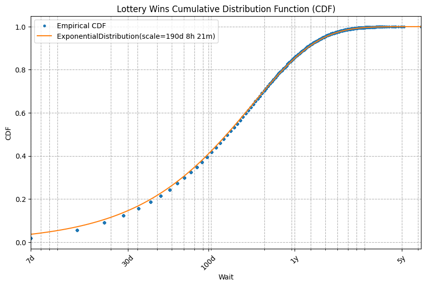
They match closely. The slight mismatch on the left is caused by the instant 7-day jump at the moment of the lottery drawing. We’ll ignore this tiny mismatch in this article.

Exponential works well on our (simulated) lottery win data. Let’s see how it works on our Popcorn and Wikipedia data. Here is the code to fit an exponential distribution to these dataframes.

_, popcorn_e_scale = expon.fit(popcorn_df['Time Delta'].dt.total_seconds(), floc=0)
popcorn_expon_dist = expon(scale=popcorn_e_scale)
print(f"Popcorn exponential median is {seconds_to_text(popcorn_expon_dist.median())}")
popcorn_expon_label = f'ExponentialDistribution(scale={seconds_to_text(popcorn_e_scale)})'
wait_cdf("Popcorn", popcorn_df, popcorn_ticks, dist=popcorn_expon_dist, dist_label=popcorn_expon_label, left=10, right=6*60, xscale='linear' )

_, wiki_e_scale = expon.fit(wiki_df['Time Delta'].dt.total_seconds(), floc=0)
wiki_expon_dist = expon(scale=wiki_e_scale)
print(f"Wiki exponential median is {seconds_to_text(wiki_expon_dist.median())}")
wiki_expon_label = f'ExponentialDistribution(scale={seconds_to_text(wiki_e_scale)})'
wait_cdf("Wiki Edits", wiki_df, wiki_wait_ticks, dist=wiki_expon_dist, dist_label=wiki_expon_label, xscale='log', left=60)

And here are the plots:

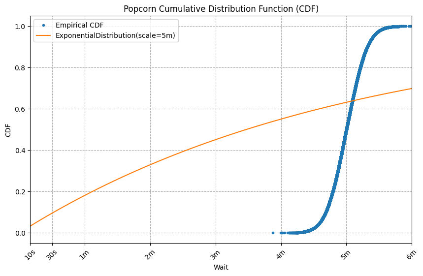
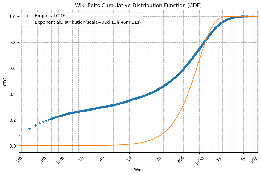
Yikes, these curve fits are terrible! The problem is that exponential distributions only model “Lottery-Win”-like data. Specifically, waits in which regardless of your wait so far, your expected wait remains the same. Because the exponential distribution fits waits that ignore your wait so far, it is called memoryless. Moreover, among continuous distributions, the exponential distribution is the only memoryless distribution.

But what if we need our distribution to have memory? The next simplest distribution to try is the Weibull distribution.

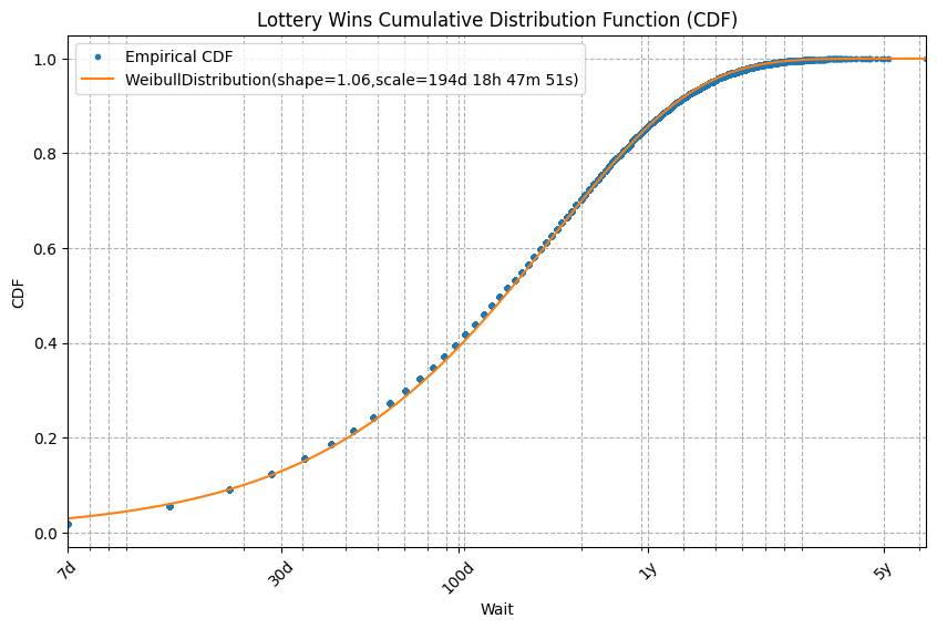
Two parameters, shape and scale parameterize a Weibull. Let’s give it a try starting with the lottery data:

from scipy.stats import weibull_min

lotto_shape, _, lotto_w_scale = weibull_min.fit(lotto_df['Time Delta'].dt.total_seconds(), floc=0)
lotto_weibull_dist = weibull_min(c=lotto_shape,scale=lotto_w_scale)

print(f"Lottery Wins Weibull median is {seconds_to_text(lotto_weibull_dist.median())}")
lotto_weibull_label = f'WeibullDistribution(shape={lotto_shape:.3},scale={seconds_to_text(lotto_w_scale)})'
wait_cdf("Lottery Wins", lotto_df, wiki_wait_ticks, dist=lotto_weibull_dist, dist_label=lotto_weibull_label, xscale='log')

This produces a fitted curve that looks like the exponential. Indeed, when shape is 1, a Weibull distribution is an exponential distribution. Here shape is 1.06.

What happens when we try to fit a Weibull to our Popcorn data?

popcorn_shape, _, popcorn_w_scale = weibull_min.fit(popcorn_df['Time Delta'].dt.total_seconds(), floc=0)
popcorn_weibull_dist = weibull_min(c=popcorn_shape, scale=popcorn_w_scale)
print(f"Popcorn Weibull median is {seconds_to_text(popcorn_weibull_dist.median())}")
popcorn_df_weibull_label = f'Weibull(shape={popcorn_shape:.3}, scale={seconds_to_text(popcorn_w_scale)})'
wait_cdf("Popcorn", popcorn_df, popcorn_ticks, dist=popcorn_weibull_dist, dist_label=popcorn_df_weibull_label, left=3*60, right=7*60, xscale='linear')

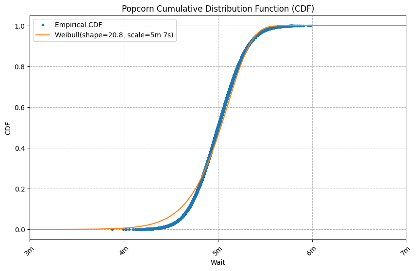
While not perfect, this fit is much better than the exponential’s fit. Notice the shape parameter’s value of 20. When a Weibull’s shape parameter is greater than 1, it indicates: “the longer you’ve waited, the less you expect to wait”.

Finally, let’s try the Weibull on the Wikipedia data.

wiki_shape, _, wiki_w_scale = weibull_min.fit(wiki_df['Time Delta'].dt.total_seconds(), floc=0)
wiki_weibull_dist = weibull_min(c=wiki_shape, scale=wiki_w_scale)
print(f"Wiki Weibull median is {seconds_to_text(wiki_weibull_dist.median())}")
wiki_df_weibull_label = f'Weibull(shape={wiki_shape:.3},scale={seconds_to_text(wiki_w_scale)})'
wait_cdf("Wiki Edits", wiki_df, wiki_wait_ticks, dist=wiki_weibull_dist, dist_label=wiki_df_weibull_label, xscale='log', left=60)

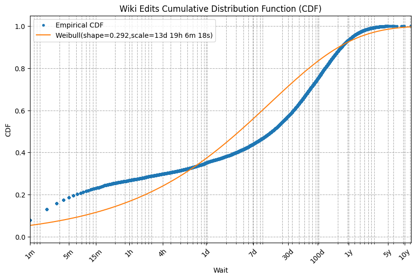
This curve fit is less than perfect, but still much better than the exponential’s fit. Notice the shape parameter value of 0.292. When a Weibull’s shape parameter is less than 1 that indicates that “the longer you’ve waited, the longer you expect to wait”. However, the Weibull is not unique in this. An infinite number of distributions also have this property. Indeed, the empirical Wikipedia distribution has this property but is not a Weibull.

Aside: I don’t know of a better simple model for the Wikipedia data. The empirical curve looks only a little more complicated than the Weibull. Perhaps we just need to identify (or invent) a slightly more general distribution with one or two additional parameters.

Conclusion

In conclusion, you and I are not (necessarily) crazy.

We have seen that there really are situations for which the longer you have waited, the longer you should expect to wait. We see it empirically in the times between Wikipedia edits. We also see it in the Weibull distribution when the shape parameter is less than 1.

Likewise, for some other waits, “The longer you’ve waited, the less you expect to wait”. We see that for popcorn. We also see it in the Weibull distribution when the shape parameter is greater than 1.

Finally, there exists a third class of waits: memoryless. For these, regardless of your wait so far, your expected wait remains the same. We saw this with the time between lottery wins. It also corresponds to a Weibull distribution with a shape parameter of 1 (which is the same as an exponential distribution).

When you have wait data to analyze, I recommend trying a Weibull distribution. Python makes fitting such a curve easy. However, if your data doesn’t fit the Weibull well, don’t use the Weibull. Instead, let your data speak for itself by using your empirical distribution directly.

Thank you for joining me on this journey into wait times. I hope you now better understand wait times and their analysis.

Please follow Carl on Medium. I write on scientific programming in Rust and Python, machine learning, and statistics. I tend to write about one article per month.

A Whimsical Journey Through Wait Times was originally published in Towards Data Science on Medium, where people are continuing the conversation by highlighting and responding to this story.