A Simple Regularization for Your GANs

How to capture data distributions effectively with GANs

In 2018, I had the privilege of orally presenting my paper at the AAAI conference. A common feedback was that the insights were clearer in the presentation than in the paper. Although some time has passed since then, I believe there’s still value in sharing the core insights and intuitions.

The paper addressed a significant problem of reliably capturing modes in a dataset with Generative Adversarial Networks (GANs). This article is formulated around my intuitions of GANs and derives the proposed approach from those intuitions. Finally, I present a copy-paste solution for those who want to try it out. If you are familiar with GANs, feel free to skip to the next section.

Paper: [Sharma, S. and Namboodiri, V., 2018, April. No modes left behind: Capturing the data distribution effectively using gans. In Proceedings of the AAAI Conference on Artificial Intelligence] (paper, github)

A quick intro to Generative Adversarial Networks

GANs are used to learn Generators for a given distribution. This means that if we are given a dataset of images, say of birds, we have to learn a function that generates images that look like birds. The Generator function is usually deterministic, so it relies on a random number as input for stochasticity to produce a variety of images. Thus, the function takes a n-dimensional number as input and outputs an image. The input number z is typically, low-dimensional and randomly sampled from a uniform or a normal distribution. This distribution is called the latent distribution Pz.

We refer to the space of “all possible” images as the data space X, the set of bird images as real R, and their distribution as Pr. The Generator at optimality, maps each value of z to some image that has a high likelihood of belonging to R.

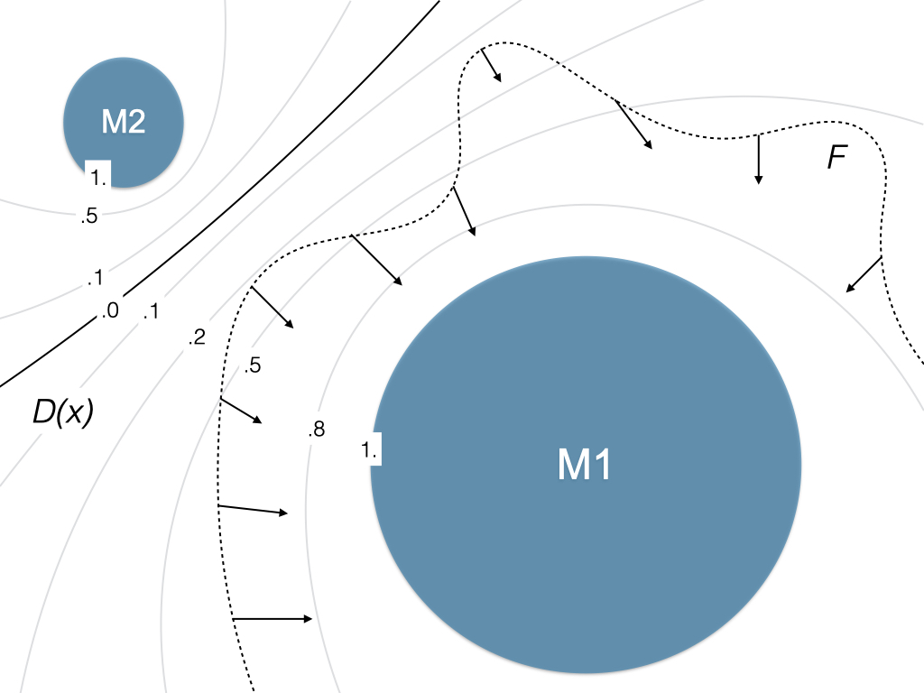
GANs solve this problem using two learned functions: a Generator (G) and a Discriminator (D). G takes the number z as input to produce a sample from data space, x = G(z). At any point, we call the set of all images generated by G as fake F, and their distribution Pg. The Discriminator takes a sample x from the data space and outputs a scalar D(x), predicting its probability of belonging to the real or fake distribution.

Initially, neither G nor D is well-trained. We sample some random numbers at each training step and pass them through G to get some fake samples. Similarly, we take an equal number of random samples from the real subset. D is trained to output 0 for fake, and 1 for real samples via cross-entropic loss. G is trained to fool D such that the output of D(G(z)) becomes 1. In other words, increase the probability of generating samples that score high (produce more), and decrease it for those that score low. The gradients flow from the loss function through D and then through G. Please refer to the original GAN paper for the loss equations.

The above figure illustrates how a GAN learns for a 1-dimensional space X. The black dotted line represents the real distribution, which we refer to as Pr. The green line represents the fake samples’ distribution Pg. The blue dotted line represents the Discriminator output D(x) for a data sample. In the beginning, neither D nor G performs correctly. First, D is updated to correctly classify real and fake samples. Next, G is updated to follow the local gradients of the Discriminator values for the generated samples D(G(z)), making Pg come closer to Pr. In other words, G slightly improves each sample based on D’s feedback. The last illustration shows the final equilibrium state.

This can be thought of as a frequentist approach. If G produces more samples from a mode than what occurs in Pr, even though the sample might look flawless, D begins to classify them as fake, discouraging G from generating such samples. Conversely, when G produces fewer samples, D begins to classify them a real, encouraging G to generate more of them. This continues till the frequency of generation of an element matches the frequency of its occurrence in Pr. Or, the element is equally likely in Pg and Pr. When the distributions exactly match, D outputs 0.5 at all points, indicating it cannot distinguish between real and fake samples. Then the loss reaches a minimum, and neither G nor D can improve further; this state is called the Nash equilibrium.

Later Wasserstein GANs modified this objective a bit. D is trained to increase for real samples and decrease for fake unboundedly. They refer to it as a Critic. Rather than computing a frequency-based loss, they modified G‘s objective to move Pg in the direction that improves D(G(z)) directly. Please refer to the original paper for the equilibrium guarantee and other details of the method.

In my experience with GANs, I’ve found it more productive to view them not as competition between G and D, but a cooperative interaction. The Discriminator’s objective is to establish a gradient of ‘realness’ between Pg and Pr, like a soft boundary. G then uses this feedback to move Pg closer to Pr. The smoother this boundary, the easier it is for G to improve. Viewing the GAN setup as competitive is disadvantageous because the loss of either networks, D or G, means failure of the final objective. However, the perspective of a joint objective aligns directly with the desired behavior.

The problem of mode loss

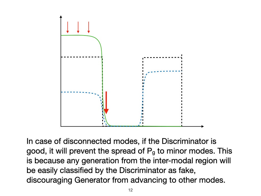
A frequently occurring problem in GANs is the losing of minor modes by the Generator. G can receive feedback by D only for the samples it generates. If G misses a mode because it initially aims for the larger modes, it never improves for it. G only improves at a mode as long as it produces samples ‘nearby’ that mode. Technically speaking, the Generator follows the local gradients from the Discriminator to shift the modes in Pg to match those of Pr. Once G loses the local gradients to a minor mode, it never faces a penalty for not generating samples from that mode. It is a problem with real-world datasets, which are usually sparse, and many minor modes occur.

This can be seen in the differential equation that is used to compute the gradients. Given the loss function, gradients for learning G are computed as:

The middle term relies on seeing an improvement in D(G(z)) wrt the data sample G(z) for the generated samples.

Our Method

In our paper, we proposed a reliable approach to solving this problem. We test it with generated toy datasets and a real-world image dataset with a massive single mode. We also test the quality of learned representations by evaluating the CIFAR score and qualitative analysis using the CelebA face dataset.

The following sections explain the underlying intuitions behind our approach.

The inverted Generator or Encoder

Let’s explore the opposite problem; given a dataset of images, we need to learn a mapping from the image to the latent distribution. Let’s assume the latent distribution is a 10-dimensional Uniform[0, 1] distribution. Thus, we construct a GAN where G is a function that takes images as input and outputs a 10-dimensional number with values in the range [0, 1]. D takes numbers from this space and outputs their “realness,” which indicates how likely it is to come from the Uniform distribution.

In this scenario, the Generator is called an Encoder (E). This can be because it learns to compress information. But is it useful?

We can visualize the Encoder’s task as assigning 10 floating numbers in the range [0, 1] to each image. This effectively places all the given images along a line of length 1, repeated for 10 different lines. Since we specify the Real distribution as Uniform, at equilibrium, the Encoder will match this distribution. Or, all the images will be uniformly spread along these 10 lines.

Assuming E has a finite capacity, meaning it cannot memorize all the patterns in the features and it is regularized such that there is continuity in outputs for inputs. Meaning, that the weights are finite and outputs cannot abruptly change for small changes in inputs. It will cause E to bring images with similar features into meaningful groups that can help it complete the task with these constraints. Thus, placing semantically closer images together in the feature space. While the features might be entangled, they yield meaningful representations.

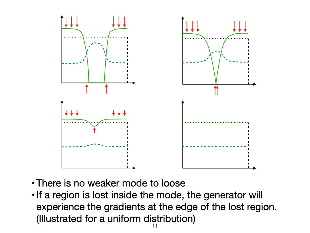
Now let’s look at the problem of mode loss from this perspective. We chose a Uniform distribution as Pr. Since it is a unimodal distribution, there is no weaker mode to lose. If E misses a region within the mode, it experiences gradients at the edge of Pg towards this region. If the Discriminator is regularized, its output will gradually change at the boundary of the missed region. Technically, D is differentiable wrt X at the boundary of this region. Then, E will follow the increasing D values to improve. Any region missed by E will eventually be captured. Thus, there can be no problem of mode loss in this case!

Since the entire region is connected, the Encoder will experience corrective gradients for any differences between Pg and Pr. There will only be a global optimum, and the network won’t get stuck in a local optimum. Thus, given enough capacity, an Encoder can perfectly encode any data distribution to a unimodal distribution. We show this for a uniform distribution here via an illustration.

From here onwards, we refer to the distribution of images as Pr, the latent distribution as Pz. The image samples will be denoted as x and the latent samples as z. The Generator takes z as input to produce images G(z), and the Encoder takes x as input to yield latent representations E(x).

BIGAN (Combined training of Encoder & Generator)

BIGAN was introduced by Donahue et al. in 2017. It simultaneously trains a Generator (G) and an Encoder (E) with a shared Discriminator (D). While the Encoder and Generator operate the same as before, the Discriminator takes both, x and z, as input and produces a scalar output.

The objective for D is to assign 1 to the tuples (x, E(x)) and assign 0 to (G(z), z). Thus, it tries to establish a boundary between the distributions of (x, E(x)) and (G(z), z). The Generator traverses this boundary gradient upwards to generate more samples labeled as 1 by the Discriminator, and the Encoder cascades down this boundary similarly. The objective of D here is to help the distributions of (x, E(x)) and (G(z), z) merge.

So what is the significance of these distributions merging? This can happen only when the distribution of G(z) matches the data distribution Pr, and the distribution of E(x) matches the latent distribution Pz. Thus, each latent variable maps to an image, and each image is mapped to a latent variable. Another inherent important feature is that this mapping is reversible, ie. G(E(x))=x and E(G(z))=z. Please refer to the original paper for more details.

Let’s visualize what it looks like — the Discriminator functions in the joint space of x and z. The illustration below shows the starting and equilibrium states of G and E, for a 1-dimensional X and a 1-dimensional Z. Pz is a uniform distribution and Pr is a sparse distribution with 5 point modes. Consequently, modes of Pr ({x1, x2, x3, x4, x5}) appear as ‘spots,’ while the latent variable’s distribution appears continuous. The green points represent the (G(z), z) tuples and the yellow points represent the (x, E(x)) tuples. Modifying E moves the yellow spots along the Z-axis, and modifying G moves the green points along the X-axis. Thus, for the distributions to match, E has to spread the yellow points along the Z-axis to approximate a uniform distribution. And, G must move the green points horizontally to resemble the distribution of given data, Pr.

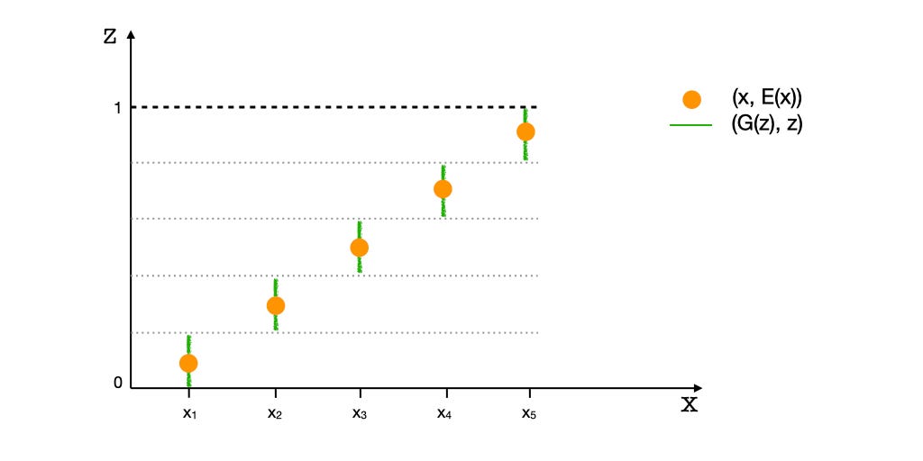
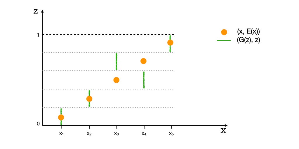
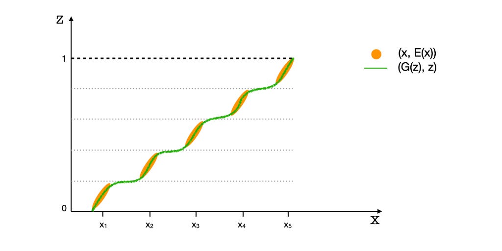
It’s important to note that G and E do not directly interact with each other, but only via D. As a result, their objectives or loss functions are independent of the other’s performance. For example, the Encoder’s objective is to make the distribution of E(x) match Pz regardless of how G is performing. This is because in matching the tuples (x, E(x)) with (G(z), z), the Encoder has control over E(x) only, and E(x) has to match Pz regardless of G(z) matching Pr. The same argument goes for the Generator. Thus, the Encoder will still perform perfectly for a unimodal distribution.

What does the problem of mode loss look like in BIGANs?

If the Generator loses the gradients to the weaker modes, they can still be lost, even if they are well Encoded.

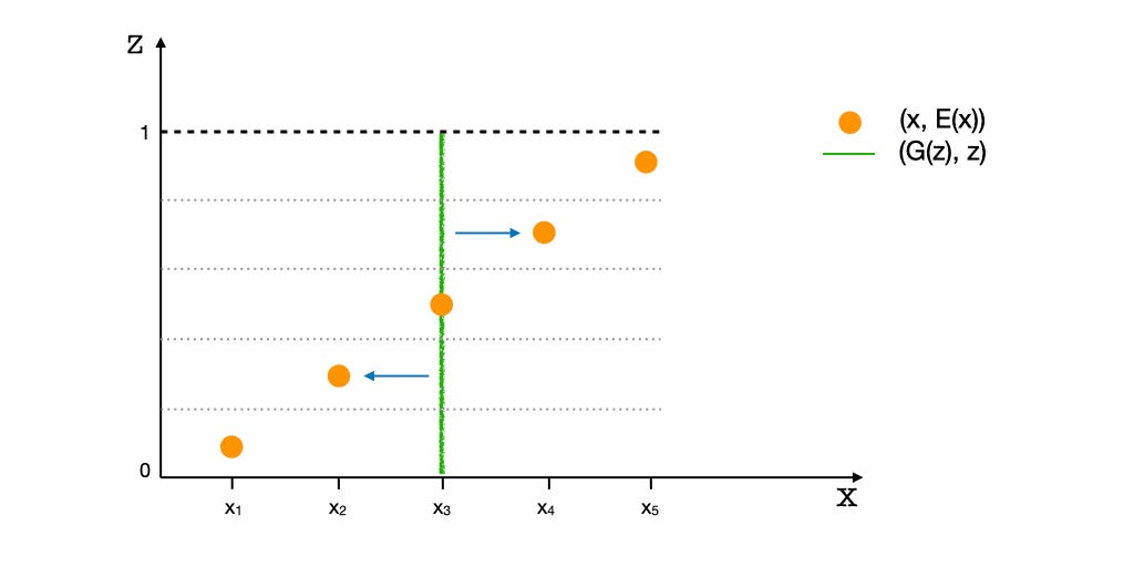
In the illustration above, G has collapsed to the mode x3. G experiences the gradients along the X-axis to the nearby modes x2 and x4, shown with blue arrows. However, the distant modes x1 and x5 may get neglected and left behind.

Finally, our solution!

An idea was proposed to stabilize Wasserstein GANs by Gulrajani et al. in the paper ‘Improved Training of Wasserstein GANs’. Since the Discriminator in WGANs is unbounded, the loss can spike if it is not regularized. This can be seen in the loss equation via expansion using the chain rule again.

Here the term ∂D/∂G should always be finite or, D(x) should be differentiable everywhere wrt x. The original method placed a bound on the weights to achieve this. However, Gulrajani et al. suggested placing a penalty on the gradients directly via an additional loss for the Discriminator. For this, points were randomly sampled between the real and generated samples from the current batch. And the magnitude of the gradients, ∂D/∂x, at those points was forced to be 1 via a mean squared loss.

The message to take away was that modeling the Discriminator landscape directly is also a viable solution. Inspired by the technique to directly model the landscape of the Discriminator, we can use something similar. Let’s have a look at Fig 7 again.

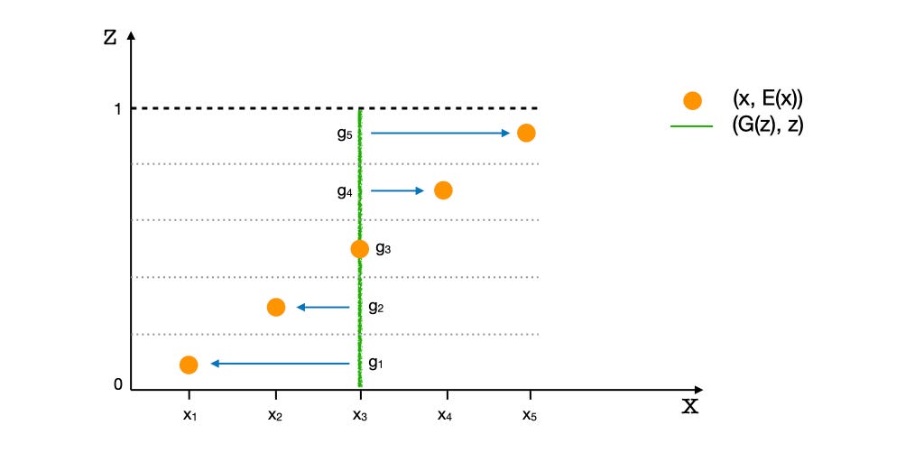
The points {g1, g2, g3, g4, g5} are the generations G(z) for the encodings E(x) of the data points in {x1, x2, x3, x4, x5} respectively or, gi = G(E(xi)). These are the reconstructions of the points xi. We need to model gradients ∂D/∂x such that the points gi start moving towards their respective target points xi.

To do this, we sample some points uniformly along the line segments connecting xi to their reconstructions gi. We then force the gradients ∂D/∂x at all those points to be unity and directed towards xi via a mean squared error. We call this pair-wise gradient penalty, and it is added as an additional loss for the Discriminator.

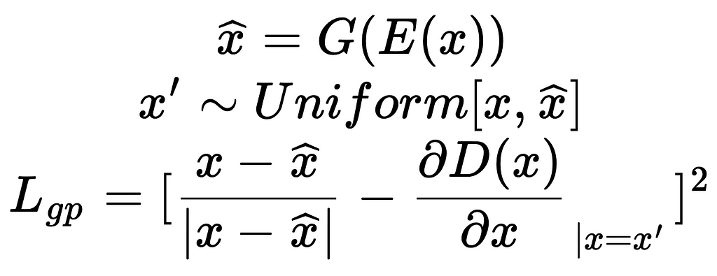
One might consider using the mean squared error between xi and its reconstruction gi as an additional loss term for the Generator, aiming for a similar effect. However, we found it difficult to balance the reconstruction loss with the adversarial loss for the Generator. This is because the adversarial and reconstruction losses are completely different in behavior and scale, making it difficult to find a constant weight that balances them effectively across datasets, toy and real. In contrast, the gradient penalty does not constrain D(x) directly but only ∂D/∂x; thus, it is not a directly competing objective for the adversarial loss and only has a regularizing effect. We found a single constant (λ=1) to work in all cases.

Does it work?

We train simple networks like DCGAN and MLPs with different losses. We use toy datasets to visualize the solution better and use an image dataset with a heavy central mode to check mode loss.

A. Toy Dataset
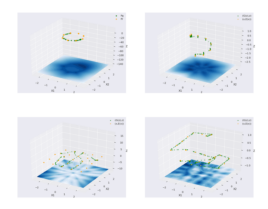
We synthesize (2-dim X and 1-dim Z) datasets with multiple sparse modes using a mixture of Normal distributions. These modes are arranged in circles and girds. It can be seen that the default BIGAN easily misses modes, but our method captured all modes in all cases.

B. Heavy central mode
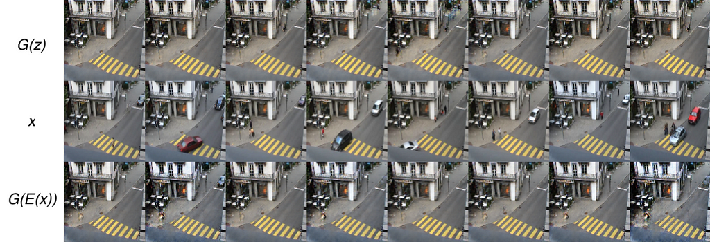
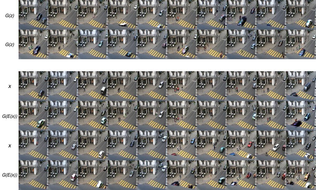
We extracted snapshots at regular intervals from footage of a traffic intersection (ref. [5]). The background remains static, and there is very little activity at certain times at certain locations in the frame. The dataset has a huge mode as the background only, without vehicles. While the original GAN and WGAN fail consistently at the task, our method shows significant learning.

C. Latent interpolations
We also tested our method with the CelebA face dataset and found that the model learned minor features that occurred only in some frames like hats, glasses, extreme face angles, etc. Please refer to the paper for the complete results.

Try it out

For those using a BIGAN or any other method where E and G are invertible, feel free to try it out. Just add the output of the following function to the Discriminator loss. The approach should work for all network architectures. As for others using traditional GANs, BIGANs could be a valuable consideration.

def gradient_penalty(x, z, x_hat, discriminator):
    """
    Computes the pair-wise gradient penalty loss for a BIGAN.
    
    Args:
        x: Samples from the real data.
        z: Samples from encoded latent distribution (= Enc(x)).
        x_hat: The reconstruction of the real samples (= G(E(x)))
        discriminator: The discriminator model with signature (x,z).
    Returns:
        gp_loss: Computed per example loss.
    """
    # Assuming only 1st dimension is the batch dimension.
    num_batch_dims = 1
    epsilon = tf.reshape(tf.random.uniform(shape=x.shape[:num_batch_dims]), x.shape[:num_batch_dims] + [1] * (len(x.shape) - num_batch_dims))
    # Compute interpolations.
    x_inter = (epsilon * x) + ((1. - epsilon) * x_hat)
    x_inter = tf.stop_gradient(x_inter)
    z = tf.stop_gradient(z)
    with tf.GradientTape(watch_accessed_variables=False) as tape:
        tape.watch(x_inter)
        # Compute discriminator values for the interpolations.
        d_inter = discriminator(x_inter, z)
    # Compute gradients at the interpolations.
    d_inter_grads = tape.gradient(d_inter, x_inter)
    # Compute the unit vector in the direction (x - x_hat).
    delta = x - x_hat
    unit_delta = delta / tf.norm(delta, axis=-1, keepdims=True)
    # Compute loss as the mse between gradients and the unit vector.
    return tf.reduce_mean((d_inter_grads - unit_delta)**2, -1)

Conclusion

If the Encoder and Discriminator have enough capacity, the Encoder can map any distribution to a unimodal latent distribution accurately. When this is achieved (and the Generator and Encoder are invertible), the Generator can also learn the real distribution perfectly via pair-wise gradient penalty. The penalty effectively regularizes the Discriminator, eliminating the need to balance the three networks. The method benefits from increasing the capacity of any one of the networks independently.

I hope this helps people get insights into GANs and maybe help with mode loss 🙂

References

[Note: Unless otherwise noted, all images are by the author]

[1] Goodfellow, I., Pouget-Abadie, J., Mirza, M., Xu, B., Warde-Farley, D., Ozair, S., Courville, A. and Bengio, Y., 2014. Generative adversarial nets. Advances in neural information processing systems, 27.
[2] Arjovsky, M., Chintala, S. and Bottou, L., 2017, July. Wasserstein generative adversarial networks. In International conference on machine learning (pp. 214–223). PMLR.
[3] Gulrajani, I., Ahmed, F., Arjovsky, M., Dumoulin, V. and Courville, A.C., 2017. Improved training of wasserstein gans. Advances in neural information processing systems, 30.
[4] Donahue, J., Krähenbühl, P. and Darrell, T., 2017. Adversarial Feature Learning. In: 5th International Conference on Learning Representations (ICLR), Toulon, France, 24–26 April 2017.
[5] (Traffic dataset): Varadarajan, J. and Odobez, J.M., 2009, September. Topic models for scene analysis and abnormality detection. In 2009 IEEE 12th International Conference on Computer Vision Workshops, ICCV Workshops (pp. 1338–1345). IEEE.

A Simple Regularization for Your GANs was originally published in Towards Data Science on Medium, where people are continuing the conversation by highlighting and responding to this story.