A Python Engineer’s Introduction To 3D Gaussian Splatting (Part 1)

Understanding and coding Gaussian Splatting from a Python Engineer’s perspective

In early 2013, authors from Université Côte d’Azur and Max-Planck-Institut für Informatik published a paper titled “3D Gaussian Splatting for Real-Time Field Rendering.”¹ The paper presented a significant advancement in real-time neural rendering, surpassing the utility of previous methods like NeRF’s.² Gaussian splatting not only reduced latency but also matched or exceeded the rendering quality of NeRF’s, taking the world of neural rendering by storm.

Gaussian splatting, while effective, can be challenging to understand for those unfamiliar with camera matrices and graphics rendering. Moreover, I found that resources for implementing gaussian splatting in Python are scarce, as even the author’s source code is written in CUDA! This tutorial aims to bridge that gap, providing a Python-based introduction to gaussian splatting for engineers versed in python and machine learning but less experienced with graphics rendering. The accompanying code on GitHub demonstrates how to initialize and render points from a COLMAP scan into a final image that resembles the forward pass in splatting applications(and some bonus CUDA code for those interested). This tutorial also has a companion jupyter notebook (part_1.ipynb in the GitHub) that has all the code needed to follow along. While we will not build a full gaussian splat scene, if followed, this tutorial should equip readers with the foundational knowledge to delve deeper into splatting technique.

To begin, we use COLMAP, a software that extracts points consistently seen across multiple images using Structure from Motion (SfM).³ SfM essentially identifies points (e.g., the top right edge of a doorway) found in more than 1 picture. By matching these points across different images, we can estimate the depth of each point in 3D space. This closely emulates how human stereo vision works, where depth is perceived by comparing slightly different views from each eye. Thus, SfM generates a set of 3D points, each with x, y, and z coordinates, from the common points found in multiple images giving us the “structure” of the scene.

In this tutorial we will use a prebuilt COLMAP scan that is available for download here (Apache 2.0 license). Specifically we will be using the Treehill folder within the downloaded dataset.

The folder consists of three files corresponding to the camera parameters, the image parameters and the actual 3D points. We will start with the 3D points.

The points file consists of thousands of points in 3D along with associated colors. The points are centered around what is called the world origin, essentially their x, y, or z coordinates are based upon where they were observed in reference to this world origin. The exact location of the world origin isn’t crucial for our purposes, so we won’t focus on it as it can be any arbitrary point in space. Instead, its only essential to know where you are in the world in relation to this origin. That is where the image file becomes useful!

Broadly speaking the image file tells us where the image was taken and the orientation of the camera, both in relation to the world origin. Therefore, the key parameters we care about are the quaternion vector and the translation vector. The quaternion vector describes the rotation of the camera in space using 4 distinct float values that can be used to form a rotation matrix (3Blue1Brown has a great video explaining exactly what quaternions are here). The translation vector then tells us the camera’s position relative to the origin. Together, these parameters form the extrinsic matrix, with the quaternion values used to compute a 3×3 rotation matrix (formula) and the translation vector appended to this matrix.

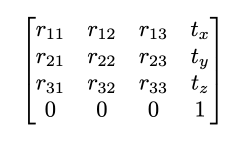
The extrinsic matrix translates points from world space (the coordinates in the points file) to camera space, making the camera the new center of the world. For example, if the camera is moved 2 units up in the y direction without any rotation, we would simply subtract 2 units from the y-coordinates of all points in order to obtain the points in the new coordinate system.

When we convert coordinates from world space to camera space, we still have a 3D vector, where the z coordinate represents the depth in the camera’s view. This depth information is crucial for determining the order of splats, which we need for rendering later on.

We end our COLMAP examination by explaining the camera parameters file. The camera file provides parameters such as height, width, focal length (x and y), and offsets (x and y). Using these parameters, we can compose the intrinsic matrix, which represents the focal lengths in the x and y directions and the principal point coordinates.

If you are completely unfamiliar with camera matrices I would point you to the First Principles of Computer Vision lectures given by Shree Nayar. Specially the Pinhole and Prospective Projection lecture followed by the Intrinsic and Extrinsic matrix lecture.

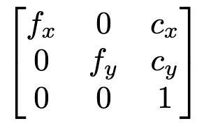
The intrinsic matrix is used to transform points from camera coordinates (obtained using the extrinsic matrix) to a 2D image plane, ie. what you see as your “image.” Points in camera coordinates alone do not indicate their appearance in an image as depth must be reflected in order to assess exactly what a camera will see.

To convert COLMAP points to a 2D image, we first project them to camera coordinates using the extrinsic matrix, and then project them to 2D using the intrinsic matrix. However, an important detail is that we use homogeneous coordinates for this process. The extrinsic matrix is 4×4, while our input points are 3×1, so we stack a 1 to the input points to make them 4×1.

Here’s the process step-by-step:

1. Transform the points to camera coordinates: multiply the 4×4 extrinsic matrix by the 4×1 point vector.
2. Transform to image coordinates: multiply the 3×4 intrinsic matrix by the resulting 4×1 vector.

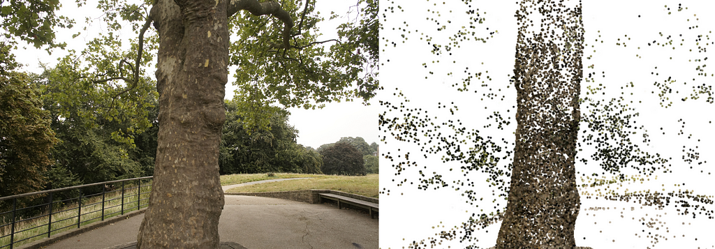
This results in a 3×1 matrix. To get the final 2D coordinates, we divide by the third coordinate of this 3×1 matrix and obtain an x and y coordinate in the image! You can see exactly how this should look about for image number 100 and the code to replicate the results is shown below.

def get_intrinsic_matrix(
    f_x: float, f_y: float, c_x: float, c_y: float
) -> torch.Tensor:
    """
    Get the homogenous intrinsic matrix for the camera
    """
    return torch.Tensor(
        [
            [f_x, 0, c_x, 0],
            [0, f_y, c_y, 0],
            [0, 0, 1, 0],
        ]
    )


def get_extrinsic_matrix(R: torch.Tensor, t: torch.Tensor) -> torch.Tensor:
    """
    Get the homogenous extrinsic matrix for the camera
    """
    Rt = torch.zeros((4, 4))
    Rt[:3, :3] = R
    Rt[:3, 3] = t
    Rt[3, 3] = 1.0
    return Rt

def project_points(
    points: torch.Tensor, intrinsic_matrix: torch.Tensor, extrinsic_matrix: torch.Tensor
) -> torch.Tensor:
    """
    Project the points to the image plane

    Args:
        points: Nx3 tensor
        intrinsic_matrix: 3x4 tensor
        extrinsic_matrix: 4x4 tensor
    """
    homogeneous = torch.ones((4, points.shape[0]), device=points.device)
    homogeneous[:3, :] = points.T
    projected_to_camera_perspective = extrinsic_matrix @ homogeneous
    projected_to_image_plane = (intrinsic_matrix @ projected_to_camera_perspective).T # Nx4
    
    x = projected_to_image_plane[:, 0] / projected_to_image_plane[:, 2]
    y = projected_to_image_plane[:, 1] / projected_to_image_plane[:, 2]
    return x, y



colmap_path = "treehill/sparse/0"
reconstruction = pycolmap.Reconstruction(colmap_path)

points3d = reconstruction.points3D
images = read_images_binary(f"{colmap_path}/images.bin")
cameras = reconstruction.cameras

all_points3d = []
all_point_colors = []

for idx, point in enumerate(points3d.values()):
    if point.track.length() >= 2:
        all_points3d.append(point.xyz)
        all_point_colors.append(point.color)

gaussians = Gaussians(
    torch.Tensor(all_points3d), 
    torch.Tensor(all_point_colors),
    model_path="point_clouds"
)

# we will examine the 100th image
image_num = 100    
image_dict = read_image_file(colmap_path)
camera_dict = read_camera_file(colmap_path)

# convert quaternion to rotation matrix
rotation_matrix = build_rotation(torch.Tensor(image_dict[image_num].qvec).unsqueeze(0))
translation = torch.Tensor(image_dict[image_num].tvec).unsqueeze(0)
extrinsic_matrix = get_extrinsic_matrix(
    rotation_matrix, translation
)
focal_x, focal_y = camera_dict[image_dict[image_num].camera_id].params[:2]
c_x, c_y = camera_dict[image_dict[image_num].camera_id].params[2:4]
intrinsic_matrix = get_intrinsic_matrix(focal_x, focal_y, c_x, c_y)

points = project_points(gaussians.points, intrinsic_matrix, extrinsic_matrix)

To review, we can now take any set of 3D points and project where they would appear on a 2D image plane as long as we have the various location and camera parameters we need! With that in hand we can move forward with understanding the “gaussian” part of gaussian splatting in part 2.

1. Kerbl, Bernhard, et al. “3d gaussian splatting for real-time radiance field rendering.” ACM Transactions on Graphics 42.4 (2023): 1–14.
2. Mildenhall, Ben, et al. “Nerf: Representing scenes as neural radiance fields for view synthesis.” Communications of the ACM 65.1 (2021): 99–106.
3. Snavely, Noah, Steven M. Seitz, and Richard Szeliski. “Photo tourism: exploring photo collections in 3D.” ACM siggraph 2006 papers. 2006. 835–846.
4. Barron, Jonathan T., et al. “Mip-nerf 360: Unbounded anti-aliased neural radiance fields.” Proceedings of the IEEE/CVF Conference on Computer Vision and Pattern Recognition. 2022.

A Python Engineer’s Introduction To 3D Gaussian Splatting (Part 1) was originally published in Towards Data Science on Medium, where people are continuing the conversation by highlighting and responding to this story.