A Guide to Clustering Algorithms

Clustering is a must-have skill set for any data scientist due to its utility and flexibility to real-world problems. This article is an overview of clustering and the different types of clustering algorithms.

What is Clustering?

Clustering is a popular unsupervised learning technique that is designed to group objects or observations together based on their similarities. Clustering has a lot of useful applications such as market segmentation, recommendation systems, exploratory analysis, and more.

While clustering is a well-known and widely used technique in the field of data science, some may not be aware of the different types of clustering algorithms. While there are just a few, it is important to understand these algorithms and how they work to get the best results for your use case.

Centroid-Based Clustering

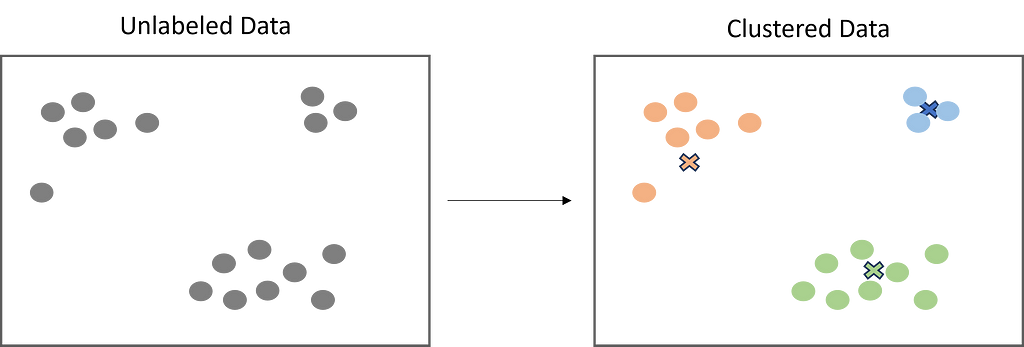
Centroid-based clustering is what most think of when it comes to clustering. It is the “traditional” way to cluster data by using a defined number of centroids (centers) to group data points based on their distance to each centroid. The centroid ultimately becomes the mean of it’s assigned data points. While centroid-based clustering is powerful, it is not robust against outliers, as outliers will need to be assigned to a cluster.

K-Means

K-Means is the most widely used clustering algorithm, and is likely the first one you will learn as a data scientist. As explained above, the objective is to minimize the sum of distances between the data points and the cluster centroid to identify the correct group that each data point should belong to. Here’s how it works:

1. A defined number of centroids are randomly dropped into the vector space of the unlabeled data (initialization).
2. Each data point measures itself to each centroid (usually using Euclidean distance) and assigns itself to the closest one.
3. The centroids relocate to the mean of their assigned data points.
4. Steps 2–3 repeat until the ‘optimal’ clusters are produced.

from sklearn.cluster import KMeans
import numpy as np

#sample data
X = np.array([[1, 2], [1, 4], [1, 0],
              [10, 2], [10, 4], [10, 0]])

#create k-means model
kmeans = KMeans(n_clusters = 2, random_state = 0, n_init = "auto").fit(X)

#print the results, use to predict, and print centers
kmeans.labels_
kmeans.predict([[0, 0], [12, 3]])
kmeans.cluster_centers_

K-Means ++

K-Means ++ is an improvement of the initialization step of K-Means. Since the centroids are randomly dropped in, there is a chance that more than one centroid might be initialized into the same cluster, resulting in poor results.

However K-Means ++ solves this by randomly assigning the first centroid that will eventually find the largest cluster. Then, the other centroids are placed a certain distance away from the initial cluster. The goal of K-Means ++ is to push the centroids as far as possible from one another. This results in high-quality clusters that are distinct and well-defined.

from sklearn.cluster import KMeans
import numpy as np

#sample data
X = np.array([[1, 2], [1, 4], [1, 0],
              [10, 2], [10, 4], [10, 0]])

#create k-means model
kmeans = KMeans(n_clusters = 2, random_state = 0, n_init = "k-means++").fit(X)

#print the results, use to predict, and print centers
kmeans.labels_
kmeans.predict([[0, 0], [12, 3]])
kmeans.cluster_centers_

Density-Based Clustering

Density-based algorithms are also a popular form of clustering. However, instead of measuring from randomly placed centroids, they create clusters by identifying high-density areas within the data. Density-based algorithms do not require a defined number of clusters, and therefore are less work to optimize.

While centroid-based algorithms perform better with spherical clusters, density-based algorithms can take arbitrary shapes and are more flexible. They also do not include outliers in their clusters and therefore are robust. However, they can struggle with data of varying densities and high dimensions.

DBSCAN

DBSCAN is the most popular density-based algorithm. DBSCAN works as follows:

1. DBSCAN randomly selects a data point and checks if it has enough neighbors within a specified radius.
2. If the point has enough neighbors, it is marked as part of a cluster.
3. DBSCAN recursively checks if the neighbors also have enough neighbors within the radius until all points in the cluster have been visited.
4. Repeat steps 1–3 until the remaining data point do not have enough neighbors in the radius.
5. Remaining data points are marked as outliers.

from sklearn.cluster import DBSCAN
import numpy as np

#sample data
X = np.array([[1, 2], [2, 2], [2, 3],
              [8, 7], [8, 8], [25, 80]])

#create model
clustering = DBSCAN(eps=3, min_samples=2).fit(X)

#print results
clustering.labels_

Hierarchical Clustering

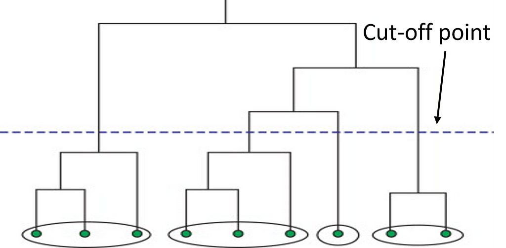
Next, we have hierarchical clustering. This method starts off by computing a distance matrix from the raw data. This distance matrix is best and often visualized by a dendrogram (see below). Data points are linked together one by one by finding the nearest neighbor to eventually form one giant cluster. Therefore, a cut-off point to identify the clusters by stopping all data points from linking together.

By using this method, the data scientist can build a robust model by defining outliers and excluding them in the other clusters. This method works great against hierarchical data, such as taxonomies. The number of clusters depends on the depth parameter and can be anywhere from 1-n.

from scipy.cluster.hierarchy import dendrogram, linkage
from sklearn.cluster import AgglomerativeClustering
from scipy.cluster.hierarchy import fcluster

#create distance matrix
linkage_data = linkage(data, method = 'ward', metric = 'euclidean', optimal_ordering = True)

#view dendrogram
dendrogram(linkage_data)
plt.title('Hierarchical Clustering Dendrogram') 
plt.xlabel('Data point') 
plt.ylabel('Distance') 
plt.show()

#assign depth and clusters
clusters = fcluster(linkage_data, 2.5, criterion = 'inconsistent', depth = 5)

Distribution Based Clustering

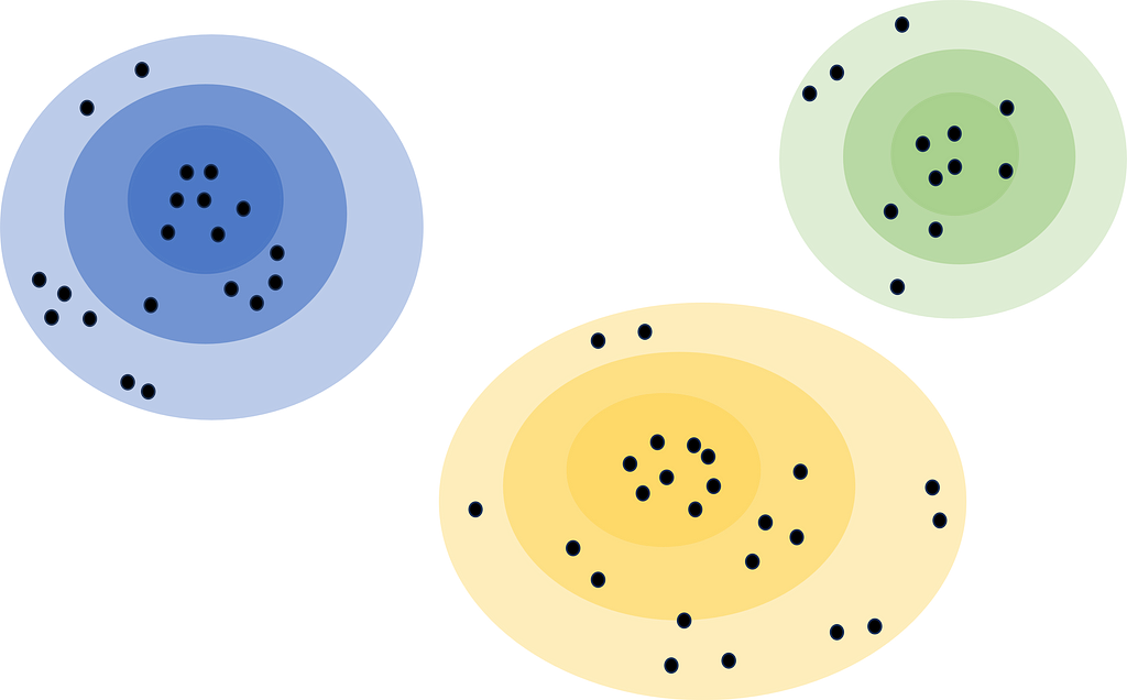
Lastly, distribution-based clustering considers a metric other than distance and density, and that is probability. Distribution-based clustering assumes that the data is made up of probabilistic distributions, such as normal distributions. The algorithm creates ‘bands’ that represent confidence intervals. The further away a data point is from the center of a cluster, the less confident we are that the data point belongs to that cluster.

Distribution-based clustering is very difficult to implement due to the assumptions it makes. It usually is not recommended unless rigorous analysis has been done to confirm its results. For example, using it to identify customer segments in a marketing dataset, and confirming these segments follow a distribution. This can also be a great method for exploratory analysis to see not only what the centers of clusters comprise of, but also the edges and outliers.

Conclusion

Clustering is an unsupervised machine learning technique that has a growing utility in many fields. It can be used to support data analysis, segmentation projects, recommendation systems, and more. Above we have explored how they work, their pros and cons, code samples, and even some use cases. I would consider experience with clustering algorithms a must-have for data scientists due to their utility and flexibility.

I hope you have enjoyed my article! Please feel free to comment, ask questions, or request other topics.

A Guide to Clustering Algorithms was originally published in Towards Data Science on Medium, where people are continuing the conversation by highlighting and responding to this story.