A Fresh Look at Nonlinearity in Deep Learning

The traditional reasoning behind why we need nonlinear activation functions is only one dimension of this story.

What do the softmax, ReLU, sigmoid, and tanh functions have in common? They’re all activation functions — and they’re all nonlinear. But why do we need activation functions in the first place, specifically nonlinear activation functions? There’s a traditional reasoning, and also a new way to look at it.

The traditional reasoning is this: without a nonlinear activation function, a deep neural network is just a composition of matrix multiplications and adding biases. These are linear transformations, and you can prove using linear algebra that the composition of linear transformations is just another linear transformation.

So no matter how many linear layers we stack together, without activation functions, our entire model is no better than a linear regression. It will completely fail to capture nonlinear relationships, even simple ones like XOR.

Enter activation functions: by allowing the model to learn a nonlinear function, we gain the ability to model all kinds of complicated real-world relationships.

This story, which you may already be familiar with, is entirely correct. But the study of any topic benefits from a variety of viewpoints, especially deep learning with all its interpretability challenges. Today I want to share with you another way to look at the need for activation functions, and what it reveals about the inner workings of deep learning models.

In short, what I want to share with you is this: the way we normally construct deep learning classifiers creates an inductive bias in the model. Specifically, using a linear layer for the output means that the rest of the model must find a linearly separable transformation of the input. The intuition behind this can be really useful, so I’ll share some examples that I hope will clarify some of this jargon.

The Traditional Explanation

Let’s revisit the traditional rationale for nonlinear activation functions with an example. We’ll look at a simple case: XOR.

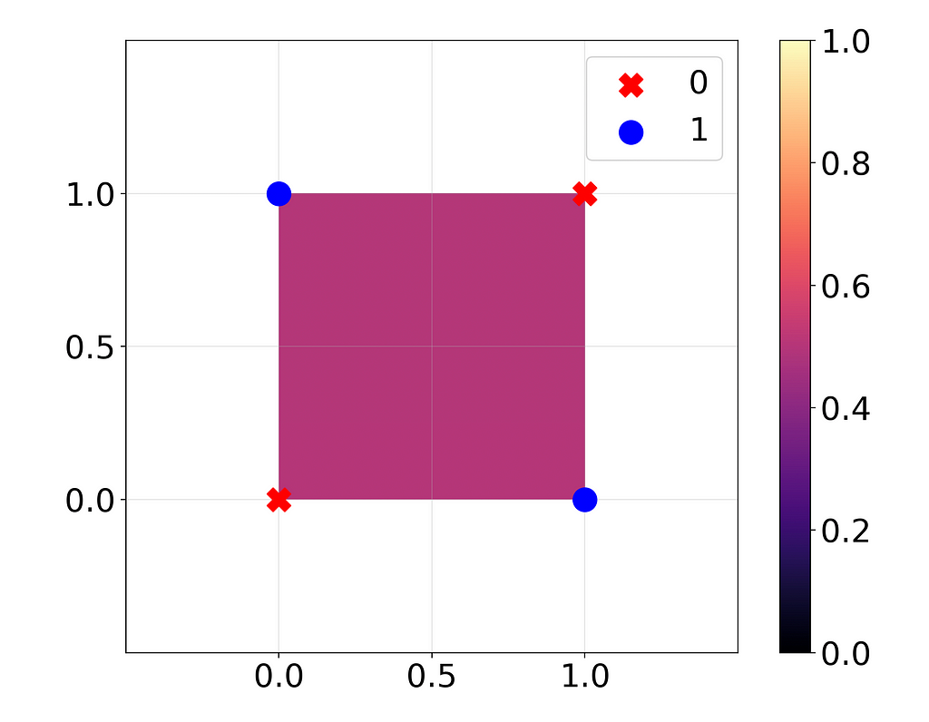
Here I’ve trained a linear regression model on the XOR function with two binary inputs (ground truth values are plotted as dots). I’ve plotted the outputs of the regression as the background color. The regression didn’t learn anything at all: it guessed 0.5 in all cases.

Now, instead of a linear model, I’m going to train a very basic deep learning model with MSE loss. Just one linear layer with two neurons, followed by the ReLU activation function, and then finally the output neuron. To keep things simple, I’ll use only weights, no biases.

What happens now?

Wow, now it’s perfect! What do the weights look like?

Layer 1 weight: [[ 1.1485, -1.1486],
                [-1.0205,  1.0189]]

(ReLU)

Layer 2 weight: [[0.8707, 0.9815]]

So for two inputs x and y, our output is:

This is really similar to

which you can verify is exactly the XOR function for inputs x, y in {0, 1}.

If we didn’t have the ReLU in there, we could simplify our model to 0.001y – 0.13x, a linear function that wouldn’t work at all. So there you have it, the traditional explanation: since XOR is an inherently nonlinear function, it can’t be precisely modeled by any linear function. Even a composition of linear functions won’t work, because that’s just another linear function. Introducing the nonlinear ReLU function allows us to capture nonlinear relationships.

Digging Deeper: Inductive Bias

Now we’re going to work on the same XOR model, but we’ll look at it through a different lens and get a better sense of the inductive bias of this model.

What is an inductive bias? Given any problem, there are many ways to solve it. Essentially, an inductive bias is something built into the architecture of a model that leads it to choose a particular method of solving a problem over any other method.

In this deep learning model, our final layer is a simple linear layer. This means our model can’t work at all unless the model’s output immediately before the final layer can be solved by linear regression. In other words, the final hidden state before the output must be linearly separable for the model to work. This inductive bias is a property of our model architecture, not the XOR function.

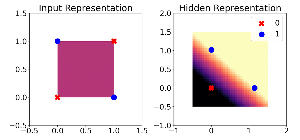
Luckily, in this model, our hidden state has only two neurons. Therefore, we can visualize it in two dimensions. What does it look like?

As we saw before, a linear regression model alone is not effective for the XOR input. But once we pass the input through the first layer and ReLU of our neural network, our output classes can be neatly separated by a line (linearly separable). This means linear regression will now work, and in fact our final layer effectively just performs this linear regression.

Now, what does this tell us about inductive bias? Since our last layer is a linear layer, the representation before this layer must be at least approximately linearly separable. Otherwise the last layer, which functions as a linear regression, will fail.

Linear Classifier Probes

For the XOR model, this might look like a trivial extension of the traditional view we saw before. But how does this work for more complex models? As models get deeper, we can get more insight by looking at nonlinearity in this way. This paper by Guillaume Alain and Yoshua Bengio investigates this idea using linear classifier probes.[1]

For many cases like MNIST handwritten digits, all the information needed to make a prediction already exists in the input: it’s just a matter of processing it. Alain and Bengio observe that as we get deeper into a model, we actually have less information at each layer, not more. But the upside is that at each layer, the information we do have becomes “easier to use”. What we mean by this is that the information becomes increasingly linearly separable after each hidden layer.

How do we find out how linearly separable the model’s representation is after each layer? Alain and Bengio suggest using what they call linear classifier probes. The idea is that after each layer, we train a linear regression to predict the final output, using the hidden states at that layer as input.

This is essentially what we did for the last XOR plot: we trained a linear regression on the hidden states right before the last layer, and we found that this regression successfully predicted the final output (1 or 0). We were unable to do this with the raw input, when the data was not linearly separable. Remember that the final layer is basically linear regression, so in a sense this method is like creating a new final layer that is shifted earlier in the model.

Alain and Bengio applied this to a convolutional neural network trained on MNIST handwritten digits: before and after each convolution, ReLU, and pooling, they added a linear probe. What they found is that the test error almost always decreased from one probe to the next, indicating an increase in linear separability.

Why does the data become linearly separable, and not “polynomially separable” or something else? Since the last layer is linear, the loss function we use will pressure all the other layers in the model to work together and create a linearly separable representation for the final layer to predict from.

Does this idea apply to large language models (LLMs) as well? In fact, it does. Jin et al. (2024) used linear classifier probes to demonstrate how LLMs learn various concepts. They found that simple concepts, such as whether a given city is the capital of a given country, become linearly separable early in the model: just a few nonlinear activations are required to model these relationships. In contrast, many reasoning skills do not become linearly separable until later in the model, or not at all for smaller models.[2]

Conclusion

When we use activation functions, we introduce nonlinearity into our deep learning models. This is certainly good to know, but we can get even more value by interpreting the consequences of linearity and nonlinearity in multiple ways.

While the above interpretation looks at the model as a whole, one useful mental model centers on the final linear layer of a deep learning model. Since this is a linear layer, whatever comes before it has to be linearly separable; otherwise, the model won’t work. Therefore, when training, the rest of the layers of the model will work together to find a linear representation that the final layer can use for its prediction.

It’s always good to have more than one intuition for the same thing. This is especially true in deep learning where models can be so black-box that any trick to gain better interpretability is helpful. Many papers have applied this intuition to get fascinating results: Alain and Bengio (2018) used it to develop the concept of linear classifier probing, while Jin et al. (2024) built on this to watch increasingly complicated concepts develop in a language model layer-by-layer.

I hope this new mental model for the purpose of nonlinearities was helpful to you, and that you’ll now be able to shed some more light on black-box deep neural networks!

References

[1] G. Alain and Y. Bengio, Understanding intermediate layers using linear classifier probes (2018), arXiv

[2] M. Jin et al., Exploring Concept Depth: How Large Language Models Acquire Knowledge at Different Layers? (2024), arXiv

A Fresh Look at Nonlinearity in Deep Learning was originally published in Towards Data Science on Medium, where people are continuing the conversation by highlighting and responding to this story.