A Benchmark and Taxonomy of Categorical Encoders

New. Comprehensive. Extendable.

A large share of datasets contain categorical features. For example, out of 665 datasets on the UC Irvine Machine Learning Repository [1], 42 are fully categorical and 366 are reported as mixed. However, distance-based ML models require features in a numerical format. Categorical encoders replace the categories in such features with real numbers.

A variety of categorical encoders exist, but there have been few attempts to compare them on many datasets, with various ML models, and in different pipelines. This article is about one of the latest benchmarks of encoders from our recent publication [2] (poster, code on GitHub). In this story, I focus on the content that complements the publication and is of practical importance. In particular, beyond the summary of our benchmark results, I will:

• Provide a list of 55 categorical encoders and the links to find their explanations and implementations for most of them.
• Explain that you can also use our code as a supplement to the Category Encoderspython module for the encoders not yet implemented there.
• Categorize the encoders into families so that you do not have to remember each individual encoder, but instead have an idea of how to build a member of each family.
• Explain how you can reuse the code from [2] and detailed benchmark data to include your encoder, dataset, or ML models in the comparison without having to re-run the existing experiments. Depending on the scope of your experiments and your computational resources, this can save you weeks of computation.

Why another benchmark?

There are already several scientific studies comparing categorical encoders [3–12] and at least one categorical encoder benchmark on TDS [13]. The study [2] that I will present here differs mainly in scope: We compared representative encoders in different configurations from a variety of encoder families. We experimented with 5 ML models (decision tree, kNN, SVM, logistic regression, LGBM), 4 quality metrics (AUC, accuracy, balanced accuracy, F1-score), 3 tuning strategies (which I will describe shortly), 50 datasets, and 32 encoder configurations.

The following table shows the encoders covered in our benchmark (the dark green column) and in other experimental comparisons (the light green columns). The blue columns show the encoders described in two additional sources: on Medium [14] and in the article dedicated to contrast encoders [15]. The last yellow column shows the encoders covered by the Category Encoders module [16]. Note that the code from [2] implements some encoders — from the similarity, binning, and data constraining families — that are not part of the Category Encoders module. In addition, we have found that the interface to the GLMM encoder implemented in R and used in [2] is much faster than the GLMM encoder from Category Encoders. Therefore, you may find our code useful for these implementations.

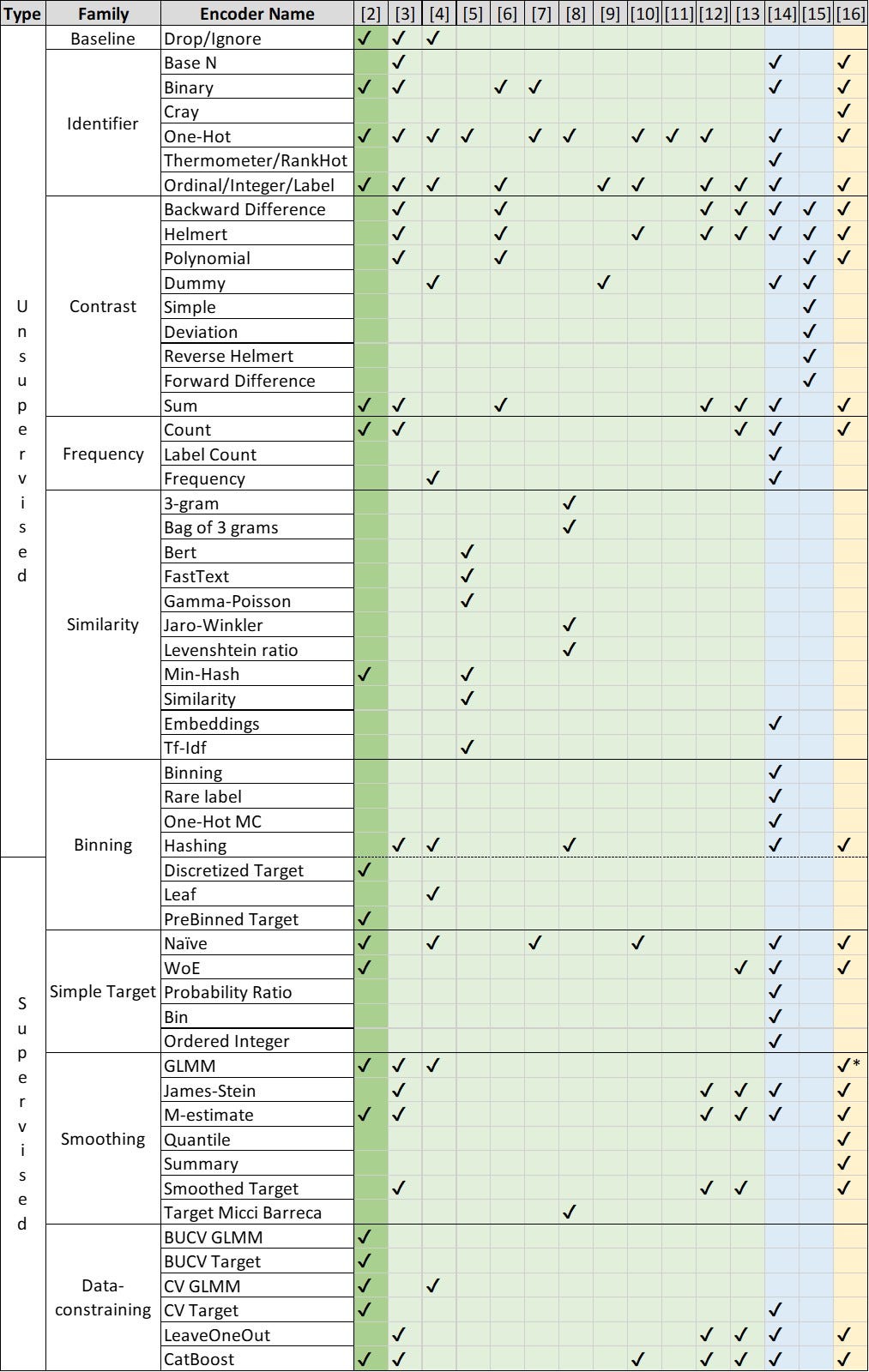
Table 1 already contains a number of encoders, and the list is by no means exhaustive. To navigate the encoder landscape, it is therefore useful to classify encoders in order to understand the principles of encoder design, rather than to memorize a large number of individual encoders.

Families of encoders

In the following, we consider a categorical feature of length n with cardinality k. At the top level, categorical encoders are supervised or unsupervised.

1. Unsupervised encoders do not include the target variable in the encoding process.

1.1. Identifier encoders transform categorical variables using a bijective function, i.e., they assign each category a unique numeric value or a unique combination of numeric values. They create from 1 up to k new features. For example, One-Hot encoder creates k features, label or ordinal encoders create a single new feature, Base N encoders create ⌈log(k)⌉ new features, where the logarithm is of base N.

These encoders are useful for categorical variables that denote unique identifiers, such as product codes or zip codes. Typically, with the exception of ordinal encoder, identifier encoders do not assume that any inherent order in the categories conveys meaningful information for analysis, and thus ignore any such order during the encoding process.

1.2. Contrast encoders transform categorical variables by assigning numerical values based on comparisons between categories. Typically, a set of k-1 new features represents a categorical variable with k categories. Unlike identifier encoders, these encoders are specifically designed to explore the relationships between different levels of a categorical variable in a regression analysis.

To create a contrast encoder, one has a choice of different coding schemes [15]. Each contrasts a category with other categories in a particular way to test a related hypothesis about the data. For example, Helmert coding contrasts each level with the mean of subsequent levels, while sum coding contrasts each level with the overall mean.

1.3. Frequency encoders replace the categories of a categorical variable with corresponding values that are a function of the frequency of those categories in the data set. Unlike identifier or contrast encoders, frequency encoders do not guarantee to assign unique identifiers and create a single new feature. They provide a numerical representation of occurrence rates, which can be particularly useful when an ML model benefits from understanding the commonality of category values. All three frequency encoders in Table 1 are monotonically increasing functions of frequency. However, this is not a necessary condition for defining this group.

1.4. Similarity encoders [5, 8, 18] transform categorical data into numerical form by applying similarity or distance metrics that capture similarities between different categories.

One group of similarity encoders [8, 18] is based on a morphological comparison between two categories treated as strings. Examples of similarity metrics are Levenshtein’s ratio, Jaro-Winkler similarity, or N-gram similarity. The categorical variable is then encoded as a vector, where each dimension corresponds to a pairwise comparison of a reference category with all categories, and the value represents the computed similarity score (similar to constructing a variance-covariance matrix). Encoders of this group typically create k new features. This encoding is particularly useful for handling “dirty” categorical datasets that may contain typos and redundancies [18]. One can think of One-Hot encoding as a special case of similarity encoding, where the similarity measure can take only two values, 0 or 1.

Another group of similarity encoders [5], including, e.g. Embeddings, Min-Hash, or Gamma-Poisson matrix factorization, is designed for high cardinality categories (k>>1). They project categorical features into a lower dimensional space. This group is thus similar to binning encoders, which are also particularly useful for large k but do not aim to preserve the morphological similarity of categories.

2. Supervised encoders use information about the target variable. For regression or binary classification tasks, they typically create a single new feature for each categorical one.

2.1. Simple target encoders capture the relationship between the categorical characteristic and the target. Constructing a simple target encoder involves calculating a statistic based on the target variable for each level of the categorical variable. Common statistics include the mean, median, or probability ratios of the target variable conditional on each category.

The procedure is as follows:

• For each category level, group the data by the categorical variable.
• Within each group, compute the desired statistic of interest.
• For each instance in the data, replace the original categorical value with the corresponding statistic.

Simple target encoding runs the risk of overfitting, especially for small data sets and categories with very few observations. Techniques such as smoothing (regularization) and cross-validation, which we describe shortly, can help mitigate this risk.

2.2. Smoothing encoders are generalizations of simple target encoders that introduce a smoothing parameter. The purpose of this smoothing parameter is to prevent overfitting and to improve the generalization of the encoder to new data, especially when there are categories with a small number of observations. A common formula for the smoothed value is

where m is the number of times the category occurs in the data set. It may slightly vary, see [13]. By adjusting the smoothing parameter, you can control the balance between the category statistic and the overall statistic. A larger smoothing parameter makes the encoding less sensitive to the category-specific target statistic. Setting the smoothing parameter to zero in the above formula results in a simple target encoding.

2.3. Data-constraining encoders use information from a subset of rows in a data set. An example of a data-constraining coder is the leave-one-out coder, which, for a given categorical value, calculates the statistic of the target variable for all other instances in which the category occurs, excluding the current instance. This approach ensures that the encoded value for a given data set does not include its own target value.

Data-constraining strategies help create encodings that are more representative of the true relationships in the unseen data and less prone to overfitting. The number of unique values in the encoded column may exceed the cardinality of the original categorical column k. One can also introduce smoothing into data-constraining encodings.

3. Binning encoders can be both supervised and unsupervised. Often, their work can be divided into two steps. The first step creates an auxiliary categorical feature by sorting the original categories into bins. The second step applies an encoder from one of the other groups discussed above to this auxiliary feature. Both steps can be either unsupervised or supervised independently of each other. For example, in the first step, you can form the bins by grouping rare categories together (unsupervised, e.g., One-Hot MC encoder); alternatively, you can apply a simple target encoder and group the categories with close encoded values together (supervised, e.g., Discretized Target encoder).

Some binning encoders, e.g. Hashing, do not have this two-stage structure. The number of new features created by binning encoders is usually <k.

Tuning strategies

Before proceeding with the results, I will briefly summarize the tuning strategies from our benchmark. This is important to understand the scope of the following figures and to reuse the data and code from our benchmark. The three tuning strategies are

No tuning:

• Encode the categorical columns of the training data;
• Train an ML model with its default hyperparameters.

Model tuning:

• Encode the categorical columns of the training data;
• Divide the training data into folds;
• Optimize the hyperparameters of an ML model using cross-validation.

Full tuning:

• Split training data into folds;
• Encode each training fold separately (in case of data constraining encoder family, each fold is further split into the nested folds);
• Optimize the hyperparameters of an ML model with cross-validation.

Results

I will name the winning encoders from our experiments, point out which tuning strategy performed best and should be part of your ML pipeline, and present the runtimes for various encoders.

Ranking

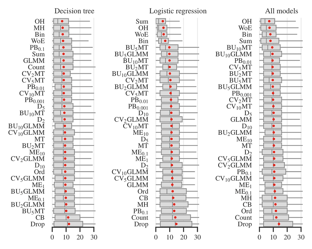
In Figure 1, the boxplots show the distribution of encoder ranks across all datasets, quality metrics, and tuning strategies. That is, each boxplot includes ~50×4×3=600 experiments for individual models and ~50×4×3×5=3000 experiments for all models, excluding the small fraction of experiments that timed out or failed for other reasons. We observed that four encoders: One-Hot, Binary (‘Bin’ on the plot), Sum, and Weight of Evidence are consistently among the best performing. For logistic regression, the difference of these four from the rest is statistically significant. This result is somewhat surprising since many previous studies (see [13, 14]) have reported drawbacks of unsupervised encoders, especially One-Hot. The exact meanings of all other encoder abbreviations on Figure 1 are not important for the rest, but you can find them in [2].

Tuning strategy

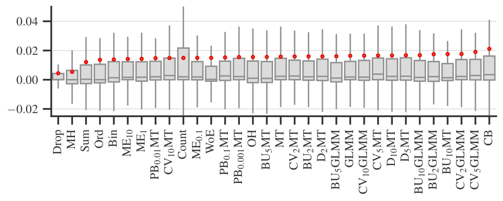
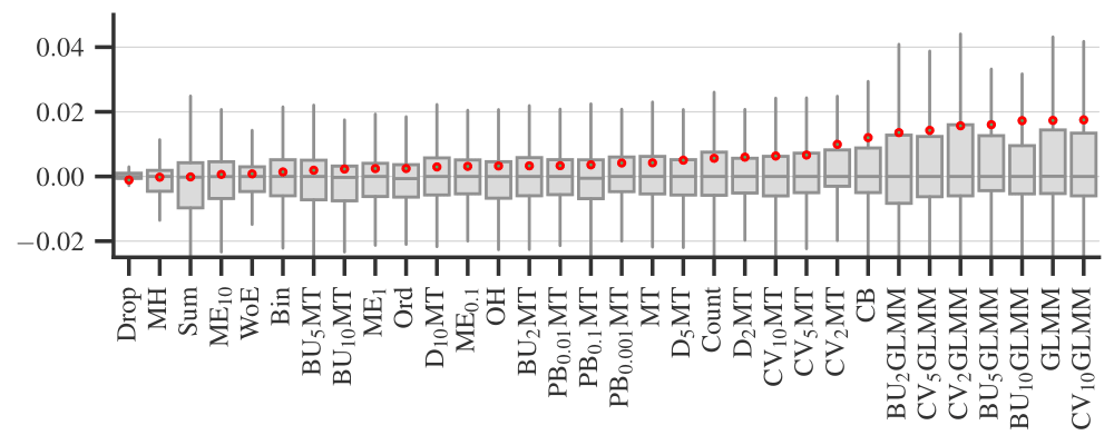
Figure 2 plots the performance difference between full and no tuning strategies (as I described above) for each categorical encoder. Each covers the experiments with different datasets, ML models, and performance metrics. Figure 3 is a similar plot comparing full and model tuning strategies. Note that these plots do not include some of the ML models and datasets because we limited the computational complexity. See [2] for details and more plots.

Based on these results, I would generally recommend sticking to the full tuning strategy, i.e., encoding data for each fold separately when optimizing the hyperparameters of an ML model; this is especially important for data constraining encoders.

Runtime

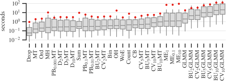
Finally, Figure 4 plots the times required to encode data sets on a logarithmic scale. Simple target and binning encoders are the fastest, while smoothing and data constraining encoders are the slowest. The four best performing encoders — One-Hot, Binary (‘Bin’ on the plot), Sum, and Weight of Evidence — take a reasonable amount of time to process data.

Reusing the code and the results

A nice feature of our benchmark is that you can easily extend it to test your approach to categorical encoding and put it in the context of existing experimental results. For example, you may want to test the encoders from Table 1 that are not part of our benchmark, or you may want to test your custom composite encoder like if n/k>a then One-Hot MC else One-Hot where k is the feature cardinality and n is the size of the dataset, as before. We explain the process on GitHub and share the demonstration of how to do this in the kaggle notebook [17]. Below is a short summary of [17].

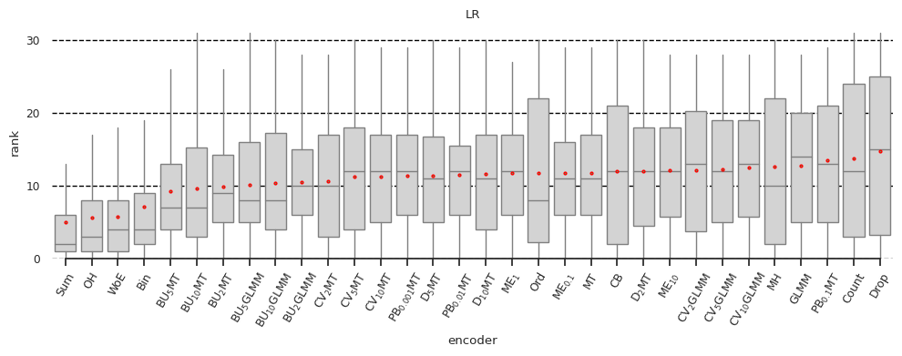
For illustrative purposes, we limited the example to a logistic regression model without hyperparameter tuning. The corresponding results of our benchmark are shown in Figure 5 below.

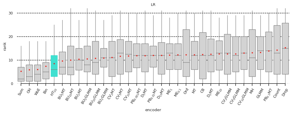
Now suppose that Yury Kashnitsky, who kindly provided feedback on our paper, wonders whether the hashing encoder is competitive with the encoders we evaluated. In [17], we show how to perform the missing experiments and find that the hashing encoder performs reasonably well with our choice of its hyperparameter, as Figure 6 shows.

Conclusion

I summarized our benchmark of categorical encoders and explained how you can benefit from our shared artifacts. You may have learned:

• Categorical encoders, as ML models, can be supervised or unsupervised.
• I presented eight families of encoders. Some encoders preserve the cardinality of categorical features, others can reduce it (often the case for binning, but also for some other encoders, e.g., Naive Target) or increase it (data constraining).
• One-Hot, Binary, Sum, and Weight of Evidence encoders performed best on average in our experiments, especially with logistic regression.
• See the kaggle notebook [17] for a demo of how to add the desired encoders to the benchmark and plot the results; the necessary code is available on GitHub.

Acknowledgements

This story would not exist if Federico Matteucci, my colleague and first author in [2], had not written the code for the benchmark and for the kaggle notebook [17].

Resources

[1] UC Irvine Machine Learning Repository
[2] Matteucci, F., Arzamasov, V., & Böhm, K. (2024). A benchmark of categorical encoders for binary classification. Advances in Neural Information Processing Systems, 36. (paper, code on GitHub, poster)
[3] Seca, D., & Mendes-Moreira, J. (2021). Benchmark of encoders of nominal features for regression. In World Conference on Information Systems and Technologies (pp. 146–155). Cham: Springer International Publishing.
[4] Pargent, F., Pfisterer, F., Thomas, J., & Bischl, B. (2022). Regularized target encoding outperforms traditional methods in supervised machine learning with high cardinality features. Computational Statistics, 37(5), 2671–2692.
[5] Cerda, P., & Varoquaux, G. (2020). Encoding high-cardinality string categorical variables. IEEE Transactions on Knowledge and Data Engineering, 34(3), 1164–1176.
[6] Potdar, K., Pardawala, T. S., & Pai, C. D. (2017). A comparative study of categorical variable encoding techniques for neural network classifiers. International journal of computer applications, 175(4), 7–9.
[7] Dahouda, M. K., & Joe, I. (2021). A deep-learned embedding technique for categorical features encoding. IEEE Access, 9, 114381–114391.
[8] Cerda, P., Varoquaux, G., & Kégl, B. (2018). Similarity encoding for learning with dirty categorical variables. Machine Learning, 107(8), 1477–1494.
[9] Wright, M. N., & König, I. R. (2019). Splitting on categorical predictors in random forests. PeerJ, 7, e6339.
[10] Gnat, S. (2021). Impact of categorical variables encoding on property mass valuation. Procedia Computer Science, 192, 3542–3550.
[11] Johnson, J. M., & Khoshgoftaar, T. M. (2021, August). Encoding techniques for high-cardinality features and ensemble learners. In 2021 IEEE 22nd international conference on information reuse and integration for data science (IRI) (pp. 355–361). IEEE.
[12] Valdez-Valenzuela, E., Kuri-Morales, A., & Gomez-Adorno, H. (2021). Measuring the effect of categorical encoders in machine learning tasks using synthetic data. In Advances in Computational Intelligence: 20th Mexican International Conference on Artificial Intelligence, MICAI 2021, Mexico City, Mexico, October 25–30, 2021, Proceedings, Part I 20 (pp. 92–107). Springer International Publishing.
[13] Benchmarking Categorical Encoders (a story on TDS)
[14] Categorical Encoding: Key Insights (my story on Medium)
[15] R Library Contrast Coding Systems for categorical variables
[16] Category Encoders (python module)
[17] Add a custom encoder to the benchmark (kaggle notebook)
[18] Similarity Encoding for Dirty Categories Using dirty_cat (a story on TDS)

A Benchmark and Taxonomy of Categorical Encoders was originally published in Towards Data Science on Medium, where people are continuing the conversation by highlighting and responding to this story.