Introducing Univariate Exemplar Recommenders: how to profile Customer Behavior in a single vector

Customer Profiling

Surveying and improving the current methodologies for customer profiling

***To understand this article, knowledge of embeddings, clustering, and recommendation systems is required. The implementation of this algorithm has been released on GitHub and is fully open-source. I am open to criticism and welcome any feedback.

Most platforms, nowadays, understand that tailoring individual choices for each customer leads to increased user engagement. Because of this, the recommender systems’ domain has been constantly evolving, witnessing the birth of new algorithms every year.

Unfortunately, no existing taxonomy is keeping track of all algorithms in this domain. While most recommendation algorithms, such as matrix factorization, employ a neural network to make recommendations based on a list of choices, in this article, I will focus on the ones that employ a vector-based architecture to keep track of user preferences.

Exemplar Recommenders

Thanks to the simplicity of embeddings, each sample that can be recommended (ex. products, content…) is converted into a vector using a pre-trained neural network (for example a matrix factorization): we can then use knn to make recommendations of similar products/customers. The algorithms following this paradigm are known as vector-based recommender systems. However, when these models take into consideration the previous user choices, they add a sequential layer to their base architecture and become technically known as vector-based sequential recommenders. Because these architectures are becoming increasingly difficult (to both remember and pronounce), I am calling them exemplar recommenders: they extract a set of representative vectors from an initial set of choices to represent a user vector.

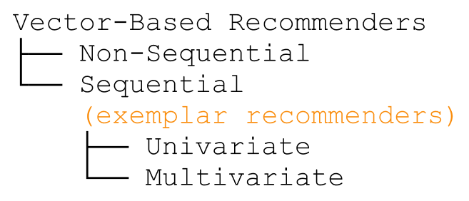
One of the first systems built on top of this architecture is Pinterest, which is running on top of its Pinnersage Recommendation engine: this scaled engine capable of managing over 2 Billion pins runs its own specific architecture and performs clustering on the choices of each individual user. As we can imagine, this represents a computational challenge when scaled. Especially after discovering covariate encoding, I would like to introduce four complementary architectures (two in particular, with the article’s name) that can relieve the stress of clustering algorithms when trying to profile each customer. You can refer to the following diagram to differentiate between them.

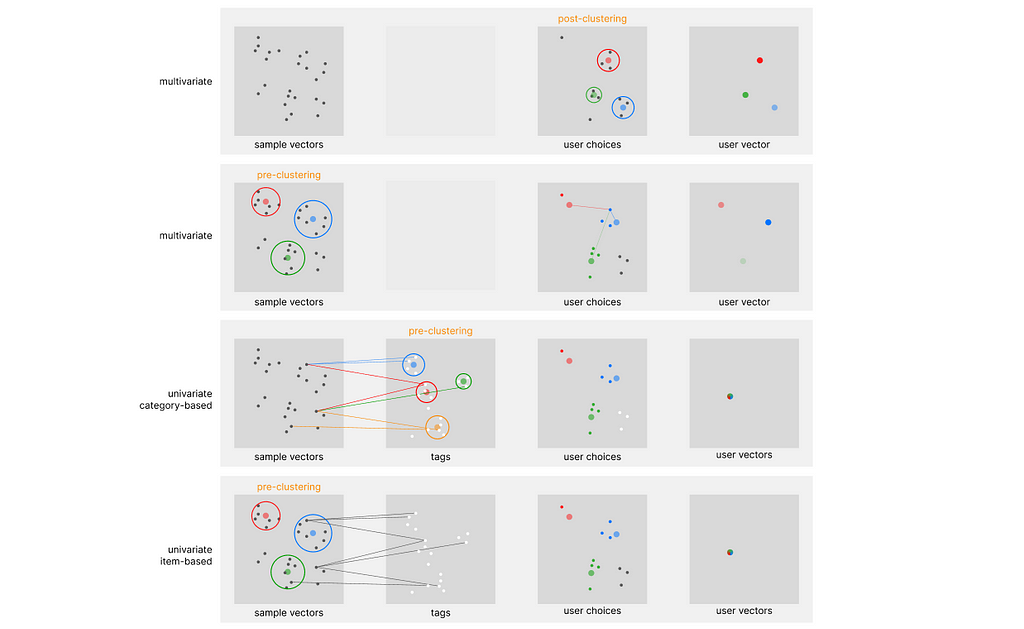
Note that all the above approaches are classified as content-based filtering, and not collaborative filtering. In regards to the exemplar architecture, we can identify two main defining parameters: in-stack clustering implementation (we either perform clustering on the sample embedding or directly on the user embedding), and the number of vectors used to store user preferences over time.

In-Stack Clustering implementation

Using once again Pinnersage as an example, we can see how it performs a novel clustering iter for each user. However advantageous from an accuracy perspective, this is computationally very heavy.

Post-Clustering

When clustering is used on top of the user embeddings, we can refer to this approach (in this specific stack) as post-clustering. However inefficient this may look, applying a non-parametric clustering algorithm on billions of samples is borderline impossible, and probably not the best option.

Pre-Clustering

There might be some use cases when applying clustering on top of the sample data could be advantageous: we can refer to this approach (in this specific stack) as pre-clustering. For example, a retail store may need to track the history of millions of users, requiring the same computational resources of the Pinnersage architecture.

However, the number of samples of a retail store, compared to the Pinterest platform, should not exceed 10.000, against the staggering 2 Billion in comparison. With such a small number of samples, performing clustering on the sample embedding is very efficient, and will relieve the need to use it on the user embedding, if utilized properly.

Introducing the Univariate Architecture

As mentioned, the biggest challenge when creating these architectures is scalability. Each user amounts to hundreds of past choices held in record that need to be computed for exemplar extraction.

Multivariate architecture

The most common way of building a vector-based recommender is to pin every user choice to an existing pre-computed vector. However, even if we resort to decay functions to minimize the number of vectors to take into account for our calculation, we still need to fill the cache with all the vectors at the time of our computation. In addition, at the time of retrieval, the vectors cannot be stored on the machine that performs the calculation, but need to be queried from a database: this sets an additional challenge for scalability.

The flow of this approach is the limited variance in recommendations. The recommended samples will be spatially very close to each other (the sample variance is minimized) and will only belong to the same category (unless there is in place a more complex logic defining this interaction).

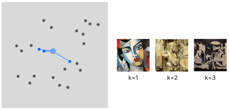
WHEN TO USE: This approach (I am only taking into account the behavior of the model, not its computational needs) is suited for applications where we can recommend a batch of samples all from the same category. Art or social media applications are one example.

Univariate architecture

With this novel approach, we can store each user choice using a single vector that keeps updating over time. This should prove to be a remarkable improvement in scalability, minimizing the computational stress derived from both knn and retrieval.

To make it even more complicated, there are two indexes where we can perform clustering. We can either cluster the items or the categories (both labeled using tags). There is no superior approach, we have to choose one depending on our use case.

> category-based

This article is entirely based on the construction of a category-based model. After tagging our data we can perform a clustering to group our data into a hierarchy of categories (in case our data is already organized into categories, there is no need to apply hierarchical clustering).

The main advantage of this approach is that the exemplar indicating the user preferences will be linked to similar categories (increasing product variance).

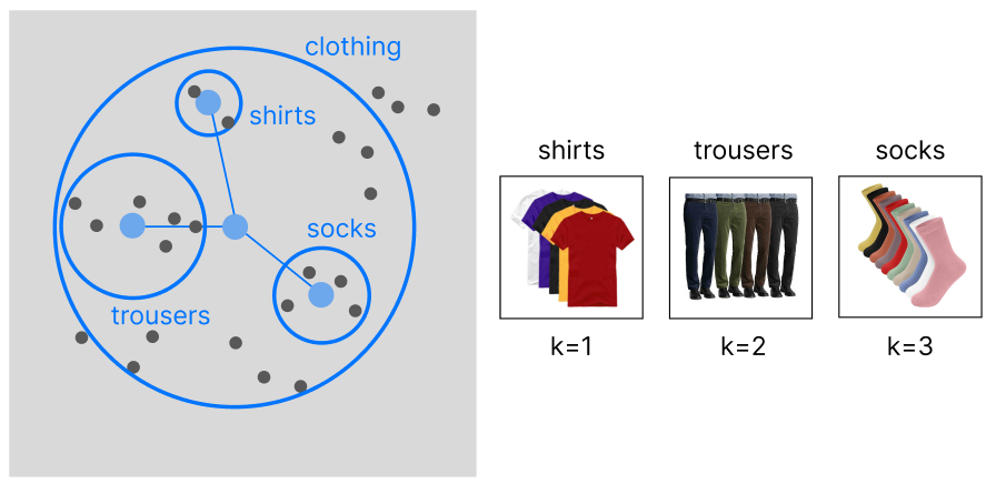
WHEN TO USE: Sometimes, we want to focus on recommending an entire category to our customers, rather than individual products. For example, if our user enjoys buying shirts (and by chance the exemplar is located in the latent region of red shirts), we would benefit more from recommending him the entire clothing category, rather than only red shirts. This approach is best suited for retail and fashion companies.

> item-based

With an item-based approach, we are performing clustering on top of our samples. This will allow us to capture more granular information on the data, rather than focusing on separated categories: we want to expand beyond the limitations of the product categorization and recommend items across existing categories.

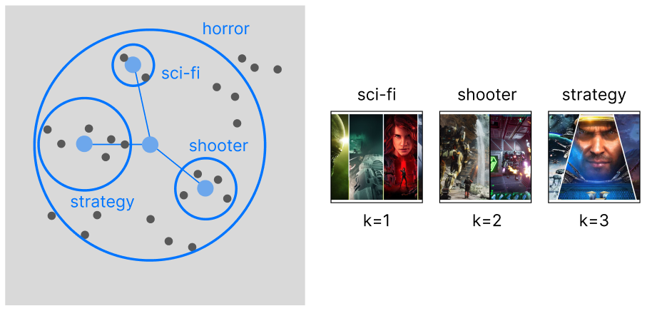
WHEN TO USE: The best companies that can make the best use for this approach are human resources and retailers with cross-categorical products (ex. videogames).

Univariate Exemplar Recommenders

Finally, we can explain in depth the architecture behind the category-based approach. This algorithm will perform exemplar extraction by only storing a single vector over time: the only technology capable of managing it is covariate encoding, hence we will use tags on top of the data. Because it uses pre-clustering, it is ideal for use cases with a manageable number of samples, but an unlimited number of users.

For this example, I will be using the open-source collection of the Steam game library (downloadable from Kaggle — MIT License), which is a perfect use case for this recommender at scale: Steam uses no more than 450 tags, and the number can occasionally increase over time; yet, it is manageable. This set of tags can be clustered very easily, and can even allow for manual intervention if we question the cluster assignment. Last, it serves millions of users, proving to be a realistic use case for our recommender.

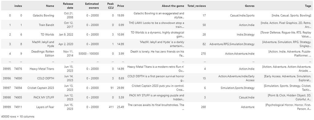
Its architecture can be articulated into the following phases:
***Note that when creating the sample code of this architecture I am using LLMs to make the entire process free from any human supervision. However, LLMs remain optional, and while they may improve the level of this recommender system, they are not an essential part of it.

1. Sample Labeling
   We need to make sure to assign tags to each of our samples. Because of semantic tag filtering, we do not need to resort to zero-shots, but we can let a LLM manage this process without any supervision.
2. Pre-Clustering
   We are going to divide the tag embedding into different clusters. For a higher level of accuracy, we are going to use hierarchical clustering with a depth of 3.
3. Cluster labeling
   Once we have defined our cluster tree, we need to label each generated supercluster. We can still use LLM for this purpose. If you decide to avoid using LLMs, not that clusters can remain in a numerical form (this may only alter the user perception of the recommender).
4. Balance non-uniform tag frequency
   The first challenge in picking from a list of tags is that the tags that appear the most (and are assigned to one cluster), heavily skew the recommender to propose that very cluster. We need to make sure that each cluster has the same probability of being recommended. We can achieve this by adding a custom multiplier that uniforms the probability of each cluster being recommended.
5. Univariate sequential encoding
   Now that our encoding weights have been defined, we can encode the user history in a vector, but with the possibility of updating it over time (using a decay function to get rid of old user preferences).
6. Account for scalability: pruning mechanism
   Because the dimensions of our vector are equivalent to the number of tags, we need to find a way to limit the size of the vector over time. PCA is a valid option, but because of the sum operations on the vector, feature pruning has proved to be more efficient.
7. Exemplar estimation
   This is where the innovation lies. We can encode the user profile as a single exemplar and still obtain separate cluster recommendations without any information loss that would arise IF we were to average multiple exemplars. This means that each of the previous multivariate methods would be incompatible with this architecture.

Let us begin with the full explanation behind the Univariate Exemplar Recommender:

1. Sample Labeling

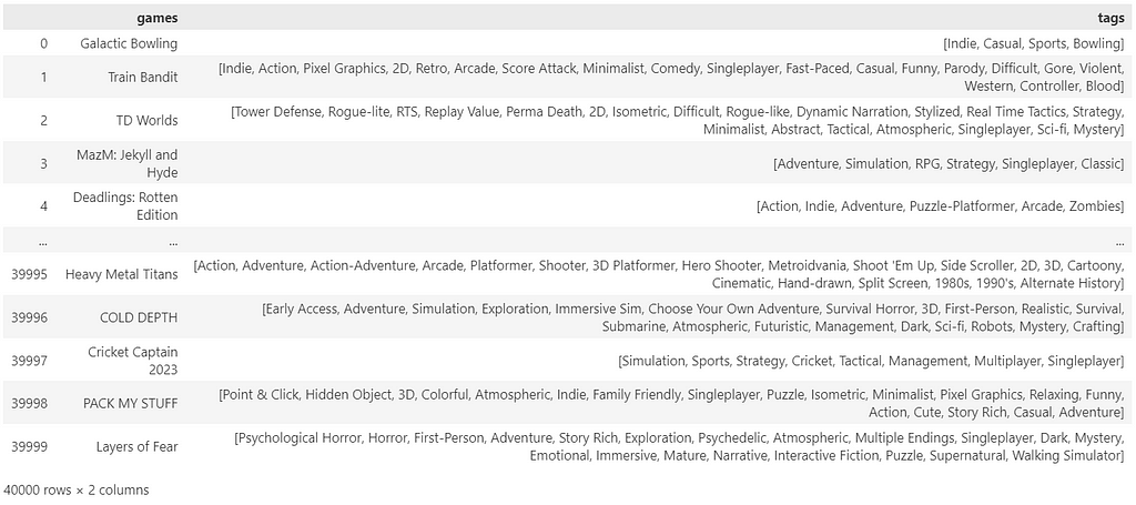
In our reference dataset all samples have already been labeled using tags. If by any chance we are working with labeled data, we can easily do that using a LLM, prompting a request for a list of tags for each sample. As explained in my article on semantic tag filtering, we do not need to use zero-shots to guide the choice of labels, and the process can be completely unsupervised.

2. Pre-Clustering

As mentioned, the idea behind this recommender is to first organize the data into clusters, and then identify the most common clusters (exemplars) that define the preferences of every single user. Because the data is ideally very small (thousands of tags against billions of samples), clustering is no longer a burden and can be done on the tag embedding, rather than on the millions of user embeddings.

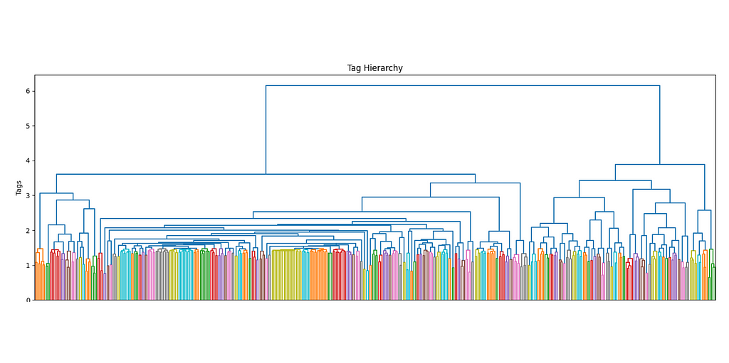
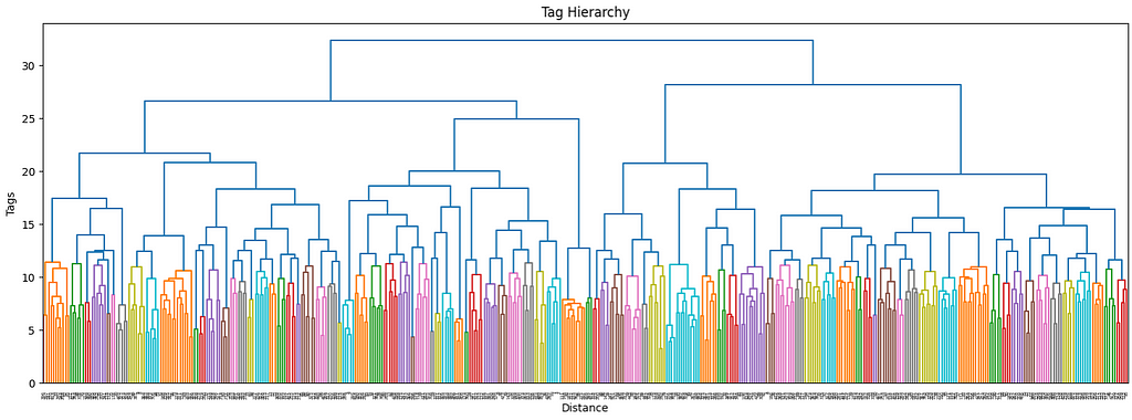
The more the number of tags increases, the more it makes sense to use a hierarchical structure to manage its complexity. Ideally, I would want not only to keep track of the main interests of each user but also their sub-interests and make recommendations accordingly. By using a dendrogram, we can define the different levels of clusters by using a threshold level.

The first superclusters (level 1) will be the result of using a threshold of 11.4, resulting in the first 81 clusters. We can also see how their distribution is non-uniform (some clusters are bigger than others), but all considered, is not excessively skewed.

The next clustering level will be defined by a smaller threshold (9), which organizes the data in 181 clusters. Equivalently for the first level of clustering, the size distribution is uneven, but there are only two big clusters, so it should not be this big of an issue.

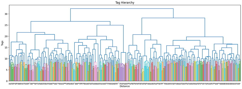
These thresholds have been arbitrarily chosen. Although there are non-parametric clustering algorithms that can perform the clustering process without any human input, they are quite challenging to manage, especially at scale, and show side effects such as the non-uniform distribution of cluster sizes. If among our clusters there are some that are too big (ex. one single cluster may even account for 20% of the overall data), then they may incorporate most recommendations without much sense.

Our priority when executing clustering is to obtain the most uniform distribution while maximizing the number of clusters so that the data can be split and differently represented as much as possible.

3. Cluster labeling

Because we have chosen to perform clustering on two levels of depths on top of our existing data, we have reached a total of 3 layers. The last layer is made by individual labels and is the only labeled layer. The other two, instead, only hold the cluster number without proper naming.

To solve this problem (note that this supercluster labeling step is not mandatory, but can improve how the user interacts with our recommender) we can use LLM on top of the superclusters.
Let us try to automatically label all our clusters by feeding the tags inside of each group:

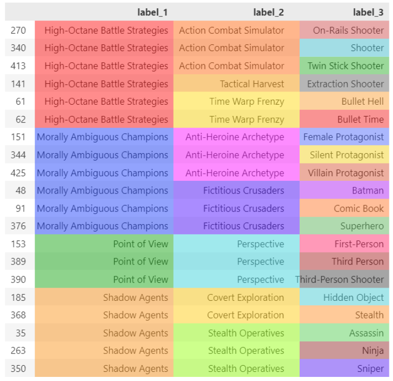
Now that also our clusters have been labeled correctly, we can start building the foundation of our sequential recommender.

4. Balance non-uniform tag frequency

So far, we have completed the easy part. Now that we have all our elements ready to create a recommender, we still need to adjust the imbalances. It would be much more intuitive to showcase this step after the recommender is done, but, unfortunately, it is part of its base structure, you will need to bear this with me.

4.1 What if we skip balancing?

Let us, for a moment, skip ahead of time, and show the capabilities of our finished recommender by simply skipping this essential step. By assigning a score of 1 to each tag, there will be some tags that are so common that they will heavily skew the recommendation scores.

The following is a Monte Carlo simulation of 5000 random tag choices from the dataset. What we are looking at is the distribution of clusters that end up being chosen randomly after summing the scores. As we can see, the distribution is highly skewed and it will certainly break the recommender in favor of the clusters with the highest score.

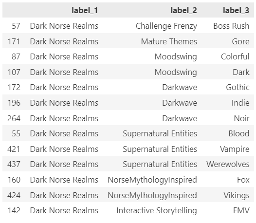
For example, the cluster “Dark Norse Realms” contains the tag Indie, which appears in 64% of all Samples (basically is almost impossible not to pick repetitively).

To be even more precise, let us directly simulate 100 different random sessions, each one picking the top 3 clusters from the session (the main user preference we keep track of), let us simulate entire user sessions so that the data is more complete. It is normal, especially when using a decay function, for the distribution to be non-uniform, and keep shifting over time.

However, if the skewness is excessive, the result is that the majority of users will be recommended the top 5% of the clusters 95% of the time (it is not precise numbers, just to prove my point).

4.2 Balancing probability distribution

Instead, let us use a proper formula for frequency adjustment. Because the probability for each cluster is different, we want to assign a score that, when used to balance the weights of our user vector, will balance cluster retrieval:

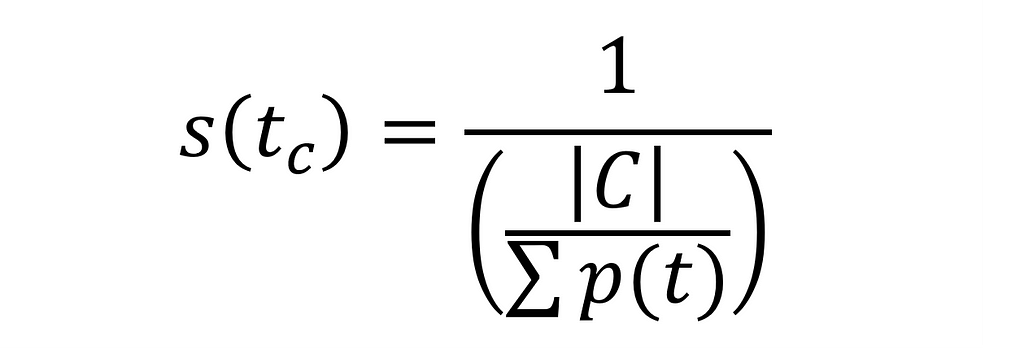
Let us look at the score assigned to each tag for 4 different random clusters:

If we apply the score to the random pick (5000 picks, counting the frequency adjusted by the aforementioned weight), we can see how the tag distribution is now balanced (the outline ~ “Adrenaline Rush” is caused by a duplicate name):

In fact, by looking at the normal distribution of the fluctuations, we see that the standard deviation for picking any cluster is approx. 0.1, which is extremely low (especially compared to before).

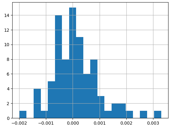
By replicating 100 sessions, we see how, even with a pseudo-uniform probability distribution, the clusters amass over time following the Pareto principle.

5. Univariate sequential encoding

It is time to build the sequential mechanism to keep track of user choices over time. The mechanism I idealized works on two separate vectors (that after the process end up being one, hence univariate), a historical vector and a caching vector.

The historical vector is the one that is used to perform knn on the existing clusters. Once a session is concluded, we update the historical vector with the new user choices. At the same time, we adjust existing values with a decay function that diminishes the existing weights over time. By doing so, we make sure to keep up with the customer trends and give more weight to new choices, rather than older ones.

Rather than updating the vector at each user makes a choice (which is not computationally efficient, in addition, we risk letting older choices decay too quickly, as every user interaction will trigger the decay mechanism), we can store a temporary vector that is only valid for the current session. Each user interaction, converted into a vector using the tag frequency as one hot weight, will be summed to the existing cached vector.

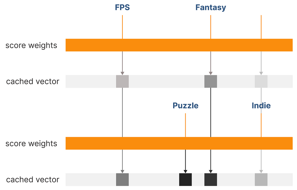
Once the session is closed, we will retrieve the historical vector from the database, merge it with the cached vector, and apply the adjustment mechanisms, such as the decay function and pruning, as we will see later). After the historical vector has been updated, it will be stored in the database replacing the old one.

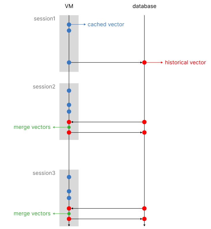
The two reasons to follow this approach are to minimize the weight difference between older and newer interactions and to make the entire process scalable and computationally efficient.

6. Pruning Mechanism

The system has been completed. However, there is an additional problem: covariate encoding has one flaw: its base vector is scaled proportionally to the number of encoded tags. For example, if our database were to reach 100k tags, the vector would have an equivalent number of dimensions.

The original covariate encoding architecture already takes this problem into account, proposing a PCA compression mechanism as a solution. However, applied to our recommender, PCA causes issues when iteratively summing vectors, resulting in information loss. Because every user choice will cause a summation of existing vectors with a new one, this solution is not advisable.

However, If we cannot compress the vector we can prune the dimensions with the lowest scores. The system will execute a knn based on the most relevant scores of the vector; this direct method of feature engineering won’t affect negatively (better yet, not excessively) the results of the final recommendation.

By pruning our vector, we can arbitrarily set a maximum number of dimensions to our vectors. Without altering the tag indexes, we can start operating on sparse vectors, rather than a dense one, a data structure that only saves the active indexes of our vectors, being able to scale indefinitely. We can compare the recommendations obtained from a full vector (dense vector) against a sparse vector (pruned vector).

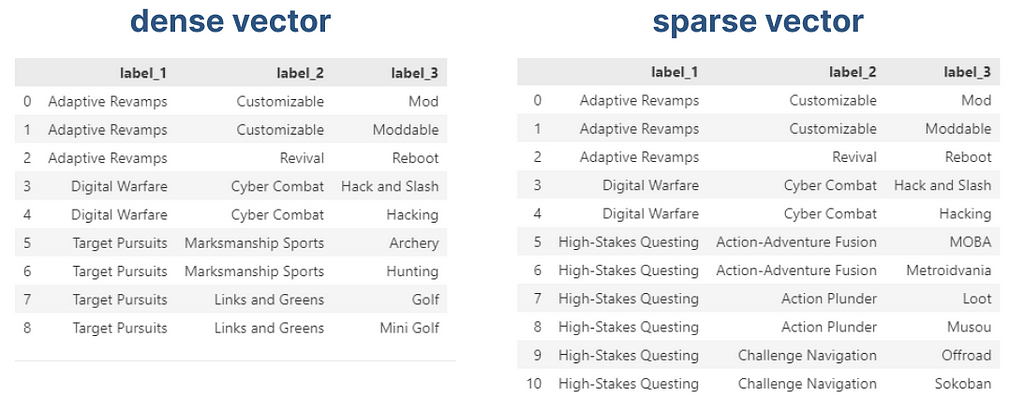
As we can see, we can spot minor differences, but the overall integrity of the vector has been maintained in exchange for scalability. A very intuitive alternative to this process is by performing clustering at the tag level, maintaining the vector size fixed. In this case, a tag will need to be assigned to the closest tag semantically, and will not occupy its dedicated dimension.

7. Exemplar estimation

Now that you have fully grasped the theory behind this new approach, we can compare them more clearly. In a multivariate approach, the first step was to identify the top user preferences using clustering. As we can see, this process required us to store as many vectors as found exemplars.

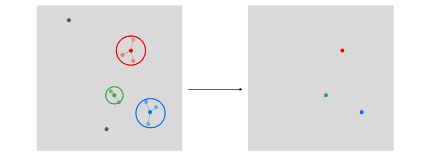
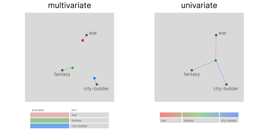
However, in a univariate approach, because covariate encoding works on a transposed version of the encoded data, we can use sections of our historical vector to store user preferences, hence only using a single vector for the entire process. Using the historical vector as a query to search through encoded tags: its top-k results from a knn search will be equivalent to the top-k preferential clusters.

8. Recommendation approaches

Now that we have captured more than one preference, how do we plan to recommend items? This is the major difference between the two systems. The traditional multivariate recommender will use the exemplar to recommend k items to a user. However, our system has assigned our customer one supercluster and the top subclusters under it (depending on our level of tag segmentation, we can increase the number of levels). We will not recommend the top k items, but the top k subclusters.

Using groupby instead of vector search

So far, we have been using a vector to store data, but that does not mean we need to rely on vector search to perform recommendations, because it will be much slower than a SQL operation. Note that obtaining the same exact results using vector search on the user array is indeed possible.

If you are wondering why you would be switching from a vector-based system to a count-based system, it is a legitimate question. The simple answer to that is that this is the most loyal replica of the multivariate system (as portrayed in the reference images), but much more scalable (it can reach up to 3000 recommendations/s on 16 CPU cores using pandas). Originally, the univariate recommender was designed to employ vector search, but, as showcased, there are simpler and better search algorithms.

Simulation

Let us run a full test that we can monitor. We can use the code from the sample notebook: for our simple example, the user selects at least one game labeled with corresponding tags.

# if no vector exists, the first choices are the historical vector
historical_vector = user_choices(5, tag_lists=[['Shooter', 'Fantasy']], tag_frequency=tag_frequency, display_tags=False)

# day1
cached_vector = user_choices(3, tag_lists=[['Puzzle-Platformer'], ['Dark Fantasy'], ['Fantasy']], tag_frequency=tag_frequency, display_tags=False)
historical_vector = update_vector(historical_vector, cached_vector, 1, 0.8)

# day2
cached_vector = user_choices(3, tag_lists=[['Puzzle'], ['Puzzle-Platformer']], tag_frequency=tag_frequency, display_tags=False)
historical_vector = update_vector(historical_vector, cached_vector, 1, 0.8)

# day3
cached_vector = user_choices(3, tag_lists=[['Adventure'], ['2D', 'Turn-Based']], tag_frequency=tag_frequency, display_tags=False)
historical_vector = update_vector(historical_vector, cached_vector, 1, 0.8)

compute_recommendation(historical_vector, label_1_max=3)

At the end of 3 sessions, these are the top 3 exemplars (label_1) extracted from our recommender:

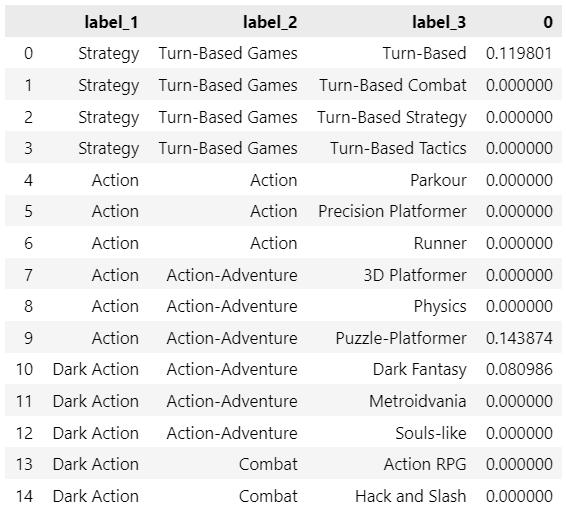
In the notebook, you will find the option to perform Monte Carlo simulations, but there would be no easy way to validate them (mostly because team games are not tagged with the highest accuracy, and I noticed that most small games list too many unrelated or common tags).

Conclusion

The architectures of the most popular recommender systems still do not take into account session history, but with the development of new algorithms and the increase in computing power, it is now possible to tackle a higher level of complexity.

This new approach should offer a comprehensive alternative to the sequential recommender systems available on the market, but I am convinced that there is always room for improvement. To further enhance this architecture it would be possible to switch from a clustering-based to a network-based approach.

It is important to note that this recommender system can only excel when applied to a limited number of domains but has the potential to shine in conditions of scarce computational resources or extremely high demand.

Introducing Univariate Exemplar Recommenders: how to profile Customer Behavior in a single vector was originally published in Towards Data Science on Medium, where people are continuing the conversation by highlighting and responding to this story.