Graph Neural Networks: Fraud Detection and Protein Function Prediction

Understanding AI applications in bio for machine learning engineers

What do a network of financial transactions and a protein structure have in common? They’re both poorly modeled in Euclidean (x, y) space and require encoding complex, large, and heterogeneous graphs to truly grok.

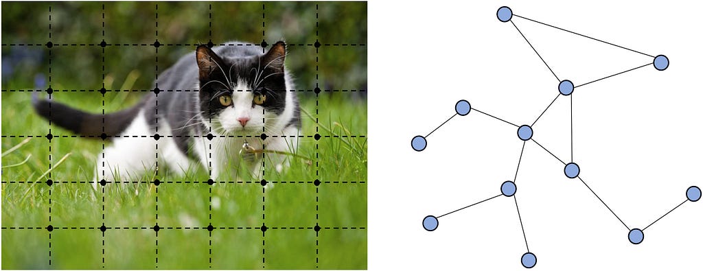
Graphs are the natural way to represent relational data in financial networks and protein structures. They capture the relationships and interactions between entities, such as transactions between accounts in financial systems or bonds and spatial proximities between amino acids in proteins. However, more widely known deep learning architectures like RNNs/CNNs and Transformers fail to model graphs effectively.

You might ask yourself why we can’t just map these graphs into 3D space? If we were to force them into a 3D grid:

• We would lose edge information, such as bond types in molecular graphs or transaction types.
• Mapping would require padding or resizing, leading to distortions.
• Sparse 3D data results would result in many unused grid cells, wasting memory and processing power.

Given these limitations, Graph Neural Networks (GNNs) serve as a powerful alternative. In this continuation of our series on Machine Learning for Biology applications, we’ll explore how GNNs can address these challenges.

As always, we’ll start with the more familiar topic of fraud detection and then learn how similar concepts are applied in biology.

Fraud Detection

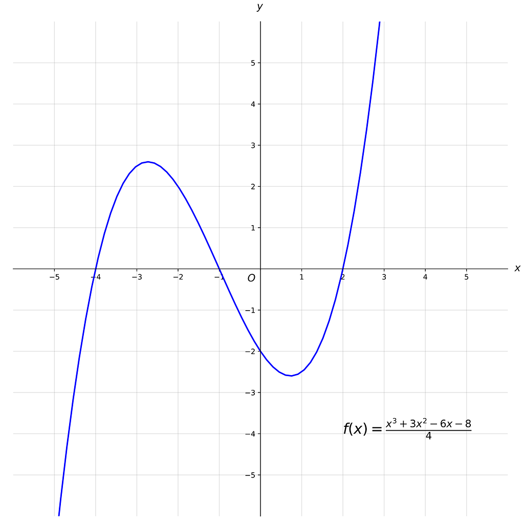
To be crystal clear, let’s first define what a graph is. We remember plotting graphs on x, y axes in grade school but what we were really doing there was graphing a function where we plotted the points of f(x)=y. We when talk about a “graph” in the context of GNNs, we mean to model pairwise relations between objects where each object is a node and the relationships are edges.

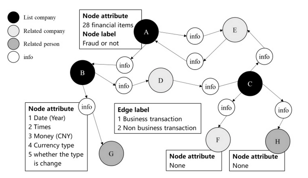
In a financial network, the nodes are accounts and the edges are the transactions. The graph would be constructed from related party transactions (RPT) and could be enriched with attributes (e.g. time, amount, currency).

Traditional rules-based and machine-learning methods often operate on a single transaction or entity. This limitation fails to account for how transactions are connected to the wider network. Because fraudsters often operate across multiple transactions or entities, fraud can go undetected.

By analyzing a graph, we can capture dependencies and patterns between direct neighbors and more distant connections. This is crucial for detecting laundering where funds are moved through multiple transactions to obscure their origin. GNNs illuminate the dense subgraphs created by laundering methods.

Message-passing frameworks

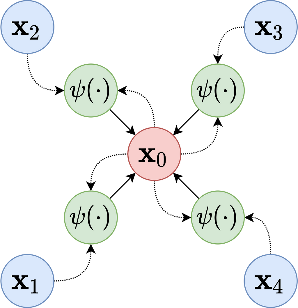
Like other deep learning methods, the goal is to create a representation or embedding from the dataset. In GNNs, these node embeddings are created using a message-passing framework. Messages pass between nodes iteratively, enabling the model to learn both the local and global structure of the graph. Each node embedding is updated based on the aggregation of its neighbors’ features.

A generalization of the framework works as follows:

• Initialization: Embeddings hv(0) are initialized with feature-based embeddings about the node, random embeddings, or pre-trained embeddings (e.g. the account name’s word embedding).
• Message Passing: At each layer t, nodes exchange messages with their neighbors. Messages are defined as features of the sender node, features of the recipient node, and features of the edge connecting them combined in a function. The combining function can be a simple concatenation with a fixed-weight scheme (used by Graph Convolutional Networks, GCNs) or attention-weighted, where weights are learned based on the features of the sender and recipient (and optionally edge features) (used by Graph Attention Networks, GATs).
• Aggregation: After the message passing step, each node aggregates the received messages (as simple as mean, max, sum).
• Update: The aggregated messages then update the node’s embedding through an update function (potentially MLPs (Multi-Layer Perceptrons) like ReLU, GRUs (Gated Recurrent Units), or attention mechanisms).
• Finalization: Embeddings are finalized, like other deep learning methods, when the representations stabilize or a maximum number of iterations is reached.

After the node embeddings are learned, a fraud score can be calculated in a few different ways:

• Classification: where the final embedding is passed into a classifier like a Multi-Layer Perceptron, which requires a comprehensive labeled historical training set.
• Anomaly Detection: where the embedding is classified as anomalous based on how distinct it is from the others. Distance-based scores or reconstruction errors can be used here for an unsupervised approach.
• Graph-Level Scoring: where embeddings are pooled into subgraphs and then fed into classifiers to detect fraud rings. (again requiring a label historical dataset)
• Label Propagation: A semi-supervised approach where label information propagates based on edge weights or graph connectivity making predictions for unlabeled nodes.

Now that we have a foundational understanding of GNNs for a familiar problem, we can turn to another application of GNNs: predicting the functions of proteins.

Protein Function Prediction

We’ve seen huge advances in protein folding prediction via AlphaFold 2 and 3 and protein design via RFDiffusion. However, protein function prediction remains challenging. Function prediction is vital for many reasons but is particularly important in biosecurity to predict if DNA will be parthenogenic before sequencing. Tradional methods like BLAST rely on sequence similarity searching and do not incoperate any structural data.

Today, GNNs are beginning to make meaningful progress in this area by leveraging graph representations of proteins to model relationships between residues and their interactions. There are considered to be well-suited for protein function prediction as well as, identifying binding sites for small molecules or other proteins and classifying enzyme families based on active site geometry.

In many examples:

• nodes are modeled as amino acid residues
• edges as the interactions between them

The rational behind this approach is a graph’s inherent ability to capture long-range interactions between residues that are distant in the sequence but close in the folded structure. This is similar to why transformer archicture was so helpful for AlphaFold 2, which allowed for parallelized computation across all pairs in a sequence.

To make the graph information-dense, each node can be enriched with features like residue type, chemical properties, or evolutionary conservation scores. Edges can optionally be enriched with attributes like the type of chemical bonds, proximity in 3D space, and electrostatic or hydrophobic interactions.

DeepFRI is a GNN approach for predicting protein functions from structure (specifically a Graph Convolutional Network (GCN)). A GCN is a specific type of GNN that extends the idea of convolution (used in CNNs) to graph data.

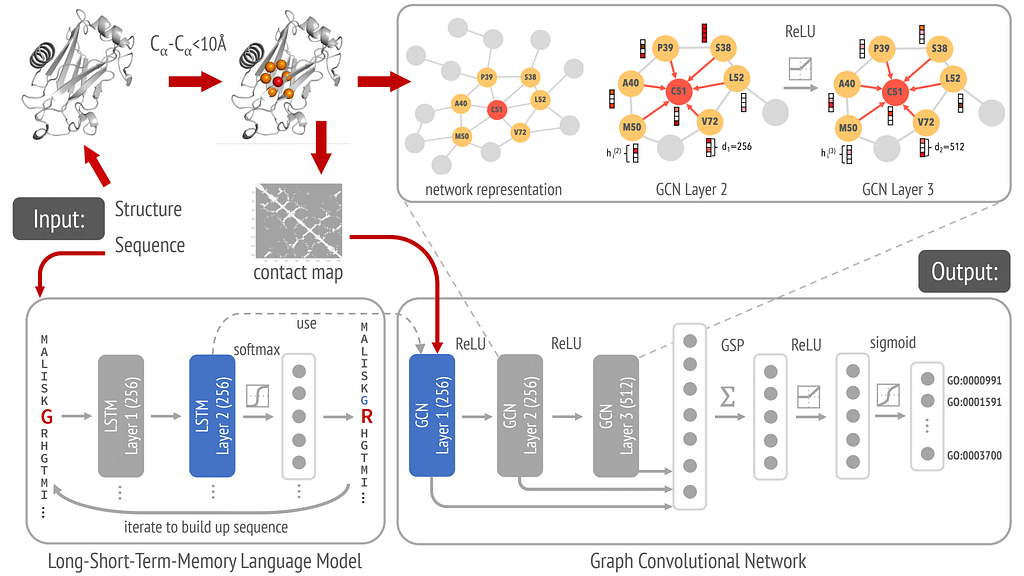
In DeepFRI, each amino acid residue is a node enriched by attributes such as:

• the amino acid type
• physicochemical properties
• evolutionary information from the MSA
• sequence embeddings from a pretrained LSTM
• structural context such as the solvent accessibility.

Each edge is defined to capture spatial relationships between amino acid residues in the protein structure. An edge exists between two nodes (residues) if their distance is below a certain threshold, typically 10 Å. In this application, there are no attributes to the edges, which serve as unweighted connections.

The graph is initialized with node features LSTM-generated sequence embeddings along with the residue-specific features and edge information created from a residue contact map.

Once the graph is defined, message passing occurs through adjacency-based convolutions at each of the three layers. Node features are aggregated from neighbors using the graph’s adjacency matrix. Stacking multiple GCN layers allows embeddings to capture information from increasingly larger neighborhoods, starting with direct neighbors and extending to neighbors of neighbors etc.

The final node embeddings are globally pooled to create a protein-level embedding, which is then used to classify proteins into hierarchically related functional classes (GO terms). Classification is performed by passing the protein-level embeddings through fully connected layers (dense layers) with sigmoid activation functions, optimized using a binary cross-entropy loss function. The classification model is trained on data derived from protein structures (e.g., from the Protein Data Bank) and functional annotations from databases like UniProt or Gene Ontology.

Final Thoughts

• Graphs are useful for modeling many non-linear systems.
• GNNs capture relationships and patterns that traditional methods struggle to model by incorporating both local and global information.
• There are many variations to GNNs but the most important (currently) are Graph Convolutional Networks and Graph Attention Networks.
• GNNs can be efficient and effective at identifying the multi-hop relationships present in money laundering schemes using supervised and unsupervised methods.
• GNNs can improve on sequence only based protein function prediction tools like BLAST by incorporating structural data. This enables researchers to predict the functions of new proteins with minimal sequence similarity to known ones, a critical step in understanding biosecurity threats and enabling drug discovery.

Cheers and if you liked this post, check out my other articles on Machine Learning and Biology.

Graph Neural Networks: Fraud Detection and Protein Function Prediction was originally published in Towards Data Science on Medium, where people are continuing the conversation by highlighting and responding to this story.