Building a Vision Inspection CNN for an Industrial Application

A step-by-step approach using PyTorch

In this article, we develop and code a Convolutional Neural Network (CNN) for a vision inspection classification task in the automotive electronics industry. Along the way, we study the concept and math of convolutional layers in depth, and we examine what CNNs actually see and which parts of the image lead them to their decisions.

Table of Content

Part 1: Conceptual background
Part 2: Defining and coding the CNN
Part 3: Using the trained model in production
Part 4: What did the CNN consider in its “decision”?

Part 1: Conceptual background

1.1 The task: Classify an industrial component as good or scrap

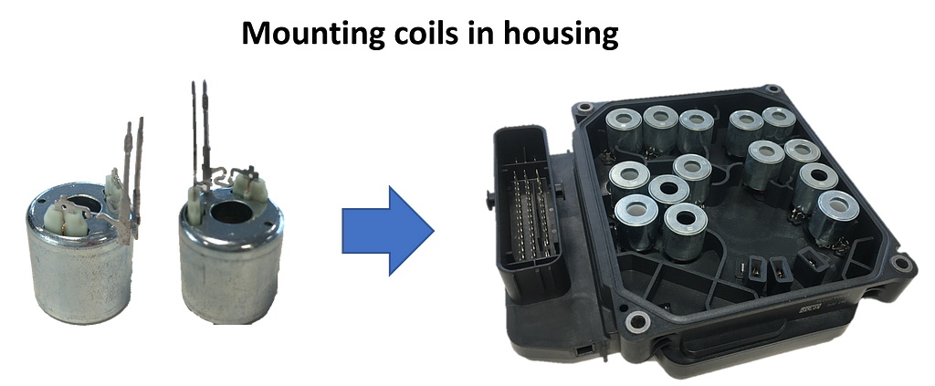
In one station of an automatic assembly line, coils with two protruding metal pins have to be positioned precisely in a housing. The metal pins are inserted into small plug sockets. In some cases, the pins are slightly bent and therefore cannot be joined by a machine. It is the task of the visual inspection to identify these coils, so that they can be sorted out automatically.

For the inspection, each coil is picked up individually and held in front of a screen. In this position, a camera takes a grayscale image. This is then examined by the CNN and classified as good or scrap.

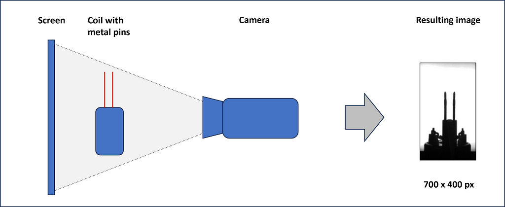
Now, we want to define a convolutional neural network that is able to process the images and learn from pre-classified labels.

1.2 What is a Convolutional Neural Network (CNN)?

Convolutional Neural Networks are a combination of convolutional filters followed by a fully connected Neural Network (NN). CNNs are often used for image processing, like face recognition or visual inspection tasks, like in our case. Convolutional filters are matrix operations that slide over the images and recalculate each pixel of the image. We will study convolutional filters later in the article. The weights of the filters are not preset (as, e.g. the sharpen function in Photoshop) but instead are learned from the data during training.

1.3 Architecture of a Convolutional Neural Network

Let’s check an example of the architecture of a CNN. For our convenience, we choose the model we will implement later.

We want to feed the CNN with our inspection images of size 400 px in height and 700 px in width. Since the images are grayscale, the corresponding PyTorch tensor is of size 1x400x700. If we used a colored image, we would have 3 incoming channels: one for red, one for green and one for blue (RGB). In this case the tensor would be 3x400x700.

The first convolutional filter has 6 kernels of size 5×5 that slide over the image and produce 6 independent new images, called feature maps, of slightly reduced size (6x396x696). The ReLU activation is not explicitly shown in Fig. 3. It does not change the dimensions of the tensors but sets all negative values to zero. ReLU is followed by the MaxPooling layer with a kernel size of 2×2. It halves the width and height of each image.

All three layers — convolution, ReLU, and MaxPooling — are implemented a second time. This finally brings us 16 feature maps with images of height 97 pixels and width 172 pixels. Next, all the matrix values are flattened and fed into the equally sized first layer of a fully connected neural network. Its second layer is already reduced to 120 neurons. The third and output layer has only 2 neurons: one represents the label “OK”, and the other the label “not OK” or “scrap”.

If you are not yet clear about the changes in the dimensions, please be patient. We study how the different kinds of layers — convolution, ReLU, and MaxPooling — work in detail and impact the tensor dimensions in the next chapters.

1.4 Convolutional filter layers

Convolutional filters have the task of finding typical structures/patterns in an image. Frequently used kernel sizes are 3×3 or 5×5. The 9, respectively 25, weights of the kernel are not specified upfront but learned during training (here we assume that we have only one input channel; otherwise, the number of weights multiply by input channels). The kernels slide over the matrix representation of the image (each input channel has its own kernel) with a defined stride in the horizontal and vertical directions. The corresponding values of the kernel and the matrix are multiplied and summed up. The summation results of each sliding position form the new image, which we call the feature map. We can specify multiple kernels in a convolutional layer. In this case, we receive multiple feature maps as the result. The kernel slides over the matrix from left to right and top to bottom. Therefore, Fig. 4 shows the kernel in its fifth sliding position (not counting the “…”). We see three input channels for the colors red, green, and blue (RGB). Each channel has one kernel only. In real applications, we often define multiple kernels per input channel.

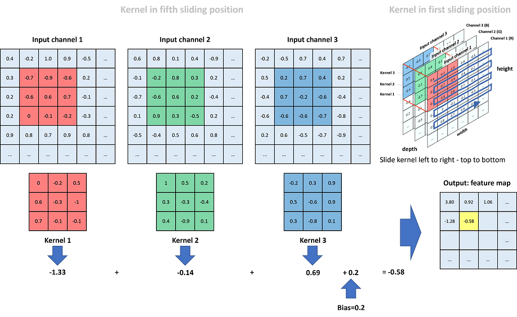
Kernel 1 does its work for the red input channel. In the shown position, we compute the respective new value in the feature map as (-0.7)*0 + (-0.9)*(-0.2) + (-0.6)*0.5 + (-0.6)*0.6 + 0.6*(-0.3) + 0.7*(-1) + 0*0.7 + (-0.1)*(-0.1) + (-0.2)*(-0.1) = (-1.33). The respective calculation for the green channel (kernel 2) adds up to -0.14, and for the blue channel (kernel 3) to 0.69. To receive the final value in the feature map for this specific sliding position, we sum up all three channel values and add a bias (bias and all kernel weights are defined during training of the CNN): (-1.33) + (-0.14) + 0.69 + 0.2 = -0.58. The value is placed in the position of the feature map highlighted in yellow.

Finally, if we compare the size of the input matrices to the size of the feature map, we see that through the kernel operations, we lost two rows in height and two columns in width.

1.5 ReLU activation layers

After the convolution, the feature maps are passed through the activation layer. Activation is required to give the network nonlinear capabilities. The two most frequently used activation methods are Sigmoid and ReLU (Rectified Linear Unit). ReLU activation sets all negative values to zero while leaving positive values unchanged.

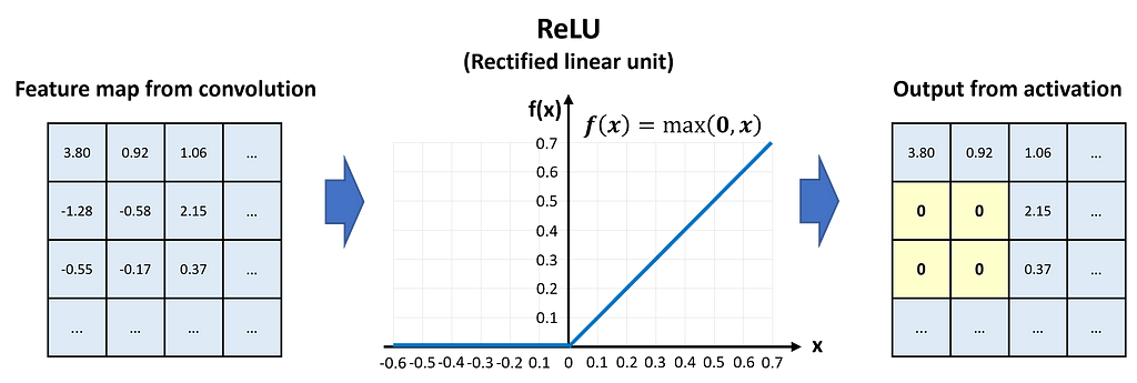
In Fig. 5, we see that the values of the feature map pass the ReLU activation element-wise.

ReLU activation has no impact on the dimensions of the feature map.

1.6 MaxPooling layers

Pooling layers have mainly the task of reducing the size of the feature maps while keeping the important information for the classification. In general, we can pool by calculating the average of an area in the kernel or returning the maximum. MaxPooling is more beneficial in most applications because it reduces the noise in the data. Typical kernel sizes for pooling are 2×2 or 3×3.

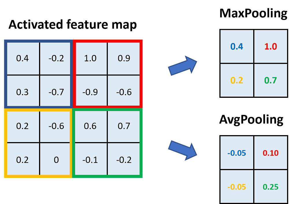
In Fig. 6, we see an example of MaxPooling and AvgPooling with a kernel size of 2×2. The feature map is divided into areas of the kernel size, and within those areas, we take either the maximum (→ MaxPooling) or the average (→ AvgPooling).

Through pooling with a kernel size of 2×2, we halve the height and width of the feature map.

1.7 Tensor dimensions in the Convolutional Neural Network

Now that we have studied the convolutional filters, the ReLU activation, and the pooling, we can revise Fig. 3 and the dimensions of the tensors. We start with an image of size 400×700. Since it is grayscale, it has only 1 channel, and the corresponding tensor is of size 1x400x700. We apply 6 convolutional filters of size 5×5 with a stride of 1×1 to the image. Each filter returns its own feature map, so we receive 6 of them. Due to the larger kernel compared to Fig. 4 (5×5 instead of 3×3), this time we lose 4 columns and 4 rows in the convolution. This means the returning tensor has the size 6x396x696.

In the next step, we apply MaxPooling with a 2×2 kernel to the feature maps (each map has its own pooling kernel). As we have learned, this reduces the maps’ dimensions by a factor of 2. Accordingly, the tensor is now of size 6x198x348.

Now we apply 16 convolutional filters of size 5×5. Each of them has a kernel depth of 6, which means that each filter provides a separate layer for the 6 channels of the input tensor. Each kernel layer slides over one of the 6 input channels, as studied in Fig. 4, and the 6 returning feature maps are added up to one. So far, we considered only one convolutional filter, but we have 16 of them. That is why we receive 16 new feature maps, each 4 columns and 4 rows smaller than the input. The tensor size is now 16x194x344.

Once more, we apply MaxPooling with a kernel size of 2×2. Since this halves the feature maps, we now have a tensor size of 16x97x172.
Finally, the tensor is flattened, which means we line up all of the 16*97*172 = 266,944 values and feed them into a fully connected neural network of corresponding size.

Part 2: Defining and coding the CNN

Conceptually, we have everything we need. Now, let’s go into the industrial use case as described in chapter 1.1.

2.1 Load the required libraries

We are going to use a couple of PyTorch libraries for data loading, sampling, and the model itself. Additionally, we load matplotlib.pyplot for visualization and PIL for transforming the images.

import torch
import torch.nn as nn
from torch.utils.data import DataLoader, Dataset
from torch.utils.data.sampler import WeightedRandomSampler
from torch.utils.data import random_split
from torchvision import datasets, transforms
import matplotlib.pyplot as plt
import numpy as np
from PIL import Image
import os
import warnings
warnings.filterwarnings("ignore")

2.2 Configure your device and specify hyperparameters

In device, we store ‘cuda’ or ‘cpu’, depending on whether or not your computer has a GPU available. minibatch_size defines how many images will be processed in one matrix operation during the training of the model. learning_rate specifies the magnitude of parameter adjustment during backpropagation, and epochs defines how often we process the whole set of training data in the training phase.

# Device configuration
device = torch.device('cuda' if torch.cuda.is_available() else 'cpu')
print(f"Using {device} device")

# Specify hyperparameters
minibatch_size = 10
learning_rate = 0.01
epochs = 60

2.3 Custom loader function

For loading the images, we define a custom_loader. It opens the images in binary mode, crops the inner 700×400 pixels of the image, loads them into memory, and returns the loaded images. As the path to the images, we define the relative path data/Coil_Vision/01_train_val_test. Please make sure that the data is stored in your working directory. You can download the files from my Dropbox as CNN_data.zip.

# Define loader function
def custom_loader(path):
    with open(path, 'rb') as f:
        img = Image.open(f)
        img = img.crop((50, 60, 750, 460))  #Size: 700x400 px
        img.load()
        return img

# Path of images (local to accelerate loading)
path = "data/Coil_Vision/01_train_val_test"

2.4 Define the datasets

We define the dataset as tuples consisting of the image data and the label, either 0 for scrap parts and 1 for good parts. The method datasets.ImageFolder() reads the labels out of the folder structure. We use a transform function to first load the image data to a PyTorch tensor (values between 0 and 1) and, second, normalize the data with the approximate mean of 0.5 and standard deviation of 0.5. After the transformation, the image data is roughly standard normal distributed (mean = 0, standard deviation = 1). We split the dataset randomly into 50% training data, 30% validation data, and 20% testing data.

# Transform function for loading
transform = transforms.Compose([transforms.ToTensor(),
                                transforms.Normalize((0.5), (0.5))])

# Create dataset out of folder structure
dataset = datasets.ImageFolder(path, transform=transform, loader=custom_loader)
train_set, val_set, test_set = random_split(dataset, [round(0.5*len(dataset)), 
                                                      round(0.3*len(dataset)), 
                                                      round(0.2*len(dataset))])

2.5 Balance the datasets

Our data is unbalanced. We have far more good samples than scrap samples. To reduce a bias towards the majority class during training, we use a WeightedRandomSampler to give higher probability to the minority class during sampling. In lbls, we store the labels of the training dataset. With np.bincount(), we count the number of 0 labels (bc[0]) and 1 labels (bc[1]). Next, we calculate probability weights for the two classes (p_nOK and p_OK) and arrange them according to the sequence in the dataset in the list lst_train. Finally, we instantiate train_sampler from WeightedRandomSampler.

# Define a sampler to balance the classes
# training dataset
lbls = [dataset[idx][1] for idx in train_set.indices]
bc = np.bincount(lbls)
p_nOK = bc.sum()/bc[0]
p_OK = bc.sum()/bc[1]
lst_train = [p_nOK if lbl==0 else p_OK for lbl in lbls]
train_sampler = WeightedRandomSampler(weights=lst_train, num_samples=len(lbls))

2.6 Define the data loaders

Lastly, we define three data loaders for the training, the validation, and the testing data. Data loaders feed the neural network with batches of datasets, each consisting of the image data and the label.
For the train_loader and the val_loader, we set the batch size to 10 and shuffle the data. The test_loader operates with shuffled data and a batch size of 1.

# Define loader with batchsize
train_loader = DataLoader(dataset=train_set, batch_size=minibatch_size, sampler=train_sampler)
val_loader = DataLoader(dataset=val_set, batch_size=minibatch_size, shuffle=True)
test_loader = DataLoader(dataset=test_set, shuffle=True)

2.7 Check the data: Plot 5 OK and 5 nOK parts

To inspect the image data, we plot five good samples (“OK”) and five scrap samples (“nOK”). To do this, we define a matplotlib figure with 2 rows and 5 columns and share the x- and the y-axis. In the core of the code snippet, we nest two for-loops. The outer loop receives batches of data from the train_loader. Each batch consists of ten images and the corresponding labels. The inner loop enumerates the batches’ labels. In its body, we check if the label equals 0 — then we plot the image under “nOK” in the second row — or if the label equals 1 — then we plot the image under “OK” in the first row. Once count_OK and count_nOK both are greater or equal 5, we break the loop, set the title, and show the figure.

# Figure and axes object
fig, axs = plt.subplots(nrows=2, ncols=5, figsize=(20,7), sharey=True, sharex=True)

count_OK = 0
count_nOK = 0

# Loop over loader batches
for (batch_data, batch_lbls) in train_loader:
    
    # Loop over batch_lbls
    for i, lbl in enumerate(batch_lbls):
        
        # If label is 0 (nOK) plot image in row 1
        if (lbl.item() == 0) and (count_nOK < 5):
            axs[1, count_nOK].imshow(batch_data[i][0], cmap='gray')
            axs[1, count_nOK].set_title(f"nOK Part#: {str(count_nOK)}", fontsize=14)
            count_nOK += 1
            
        # If label is 1 (OK) plot image in row 0
        elif (lbl.item() == 1) and (count_OK < 5):
            axs[0, count_OK].imshow(batch_data[i][0], cmap='gray')
            axs[0, count_OK].set_title(f"OK Part#: {str(count_OK)}", fontsize=14)
            count_OK += 1
    
    # If both counters are >=5 stop looping
    if (count_OK >=5) and (count_nOK >=5):
        break
        
# Config the plot canvas
fig.suptitle("Sample plot of OK and nonOK Parts", fontsize=24)
plt.setp(axs, xticks=[], yticks=[]) 
plt.show()

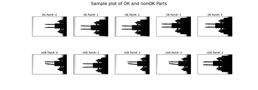
In Fig. 7, we see that most of the nOK samples are clearly bent, but a few are not really distinguishable by eye (e.g., lower right sample).

2.8 Define the CNN model

The model corresponds to the architecture depicted in Fig. 3. We feed the grayscale image (only one channel) into the first convolutional layer and define 6 kernels of size 5 (equals 5×5). The convolution is followed by a ReLU activation and a MaxPooling with a kernel size of 2 (2×2) and a stride of 2 (2×2). All three operations are repeated with the dimensions shown in Fig. 3. In the final block of the __init__() method, the 16 feature maps are flattened and fed into a linear layer of equivalent input size and 120 output nodes. It is ReLU activated and reduced to only 2 output nodes in a second linear layer.
In the forward() method, we simply call the model layers and feed in the x tensor.

class CNN(nn.Module):

    def __init__(self):
        super().__init__()

        # Define model layers
        self.model_layers = nn.Sequential(

            nn.Conv2d(in_channels=1, out_channels=6, kernel_size=5),
            nn.ReLU(),
            nn.MaxPool2d(kernel_size=2, stride=2),

            nn.Conv2d(in_channels=6, out_channels=16, kernel_size=5),
            nn.ReLU(),
            nn.MaxPool2d(kernel_size=2, stride=2),

            nn.Flatten(),
            nn.Linear(16*97*172, 120),
            nn.ReLU(),
            nn.Linear(120, 2)
        )
        
    def forward(self, x):
        out = self.model_layers(x)
        return out

2.9 Instantiate the model and define the loss function and the optimizer

We instantiate model from the CNN class and push it either on the CPU or on the GPU. Since we have a classification task, we choose the CrossEntropyLoss function. For managing the training process, we call the Stochastic Gradient Descent (SGD) optimizer.

# Define model on cpu or gpu
model = CNN().to(device)

# Loss and optimizer
loss = nn.CrossEntropyLoss()

optimizer = torch.optim.SGD(model.parameters(), lr=learning_rate)

2.10 Check the model’s size

To get an idea of our model’s size in terms of parameters, we iterate over model.parameters() and sum up, first, all model parameters (num_param) and, second, those parameters that will be adjusted during backpropagation (num_param_trainable). Finally, we print the result.

# Count number of parameters / thereof trainable
num_param = sum([p.numel() for p in model.parameters()])
num_param_trainable = sum([p.numel() for p in model.parameters() if p.requires_grad == True])

print(f"Our model has {num_param:,} parameters. Thereof trainable are {num_param_trainable:,}!")

The print out tells us that the model has more than 32 million parameters, thereof all trainable.

2.11 Define a function for validation and testing

Before we start the model training, let’s prepare a function to support the validation and testing. The function val_test() expects a dataloader and the CNN model as parameters. It turns off the gradient calculation with torch.no_grad() and iterates over the dataloader. With one batch of images and labels at hand, it inputs the images into the model and determines the model’s predicted classes with output.argmax(1) over the returned logits. This method returns the indices of the largest values; in our case, this represents the class indices.
We count and sum up the correct predictions and save the image data, the predicted class, and the labels of the wrong predictions. Finally, we calculate the accuracy and return it together with the misclassified images as the function’s output.

def val_test(dataloader, model):
    # Get dataset size
    dataset_size = len(dataloader.dataset)
    
    # Turn off gradient calculation for validation
    with torch.no_grad():
        # Loop over dataset
        correct = 0
        wrong_preds = []
        for (images, labels) in dataloader:
            images, labels = images.to(device), labels.to(device)
            
            # Get raw values from model
            output = model(images)
            
            # Derive prediction
            y_pred = output.argmax(1)
            
            # Count correct classifications over all batches
            correct += (y_pred == labels).type(torch.float32).sum().item()
            
            # Save wrong predictions (image, pred_lbl, true_lbl)
            for i, _ in enumerate(labels):
                if y_pred[i] != labels[i]:
                    wrong_preds.append((images[i], y_pred[i], labels[i]))

        # Calculate accuracy
        acc = correct / dataset_size
        
    return acc, wrong_preds

2.12 Model training

The model training consists of two nested for-loops. The outer loop iterates over a defined number of epochs, and the inner loop enumerates the train_loader. The enumeration returns a batch of image data and the corresponding labels. The image data (images) is passed to the model, and we receive the model’s response logits in outputs. outputs and the true labels are passed to the loss function. Based on loss l, we perform backpropagation and update the parameter with optimizer.step. outputs is a tensor of dimension batchsize x output nodes, in our case 10 x 2. We receive the model’s prediction through the indices of the max values over the rows, either 0 or 1.

Finally, we count the number of correct predictions (n_correct), the true OK parts (n_true_OK), and the number of samples (n_samples). Each second epoch, we calculate the training accuracy, the true OK share, and call the validation function (val_test()). All three values are printed for information purpose during the training run. With the last line of code, we save the model with all its parameters in “model.pth”.

acc_train = {}
acc_val = {}
# Iterate over epochs
for epoch in range(epochs):

    n_correct=0; n_samples=0; n_true_OK=0
    for idx, (images, labels) in enumerate(train_loader):
        model.train()
        # Push data to gpu if available
        images, labels = images.to(device), labels.to(device)
        
        # Forward pass
        outputs = model(images)
        l = loss(outputs, labels)
              
        # Backward and optimize
        optimizer.zero_grad()
        l.backward()
        optimizer.step()

        # Get prediced labels (.max returns (value,index))
        _, y_pred = torch.max(outputs.data, 1)

        # Count correct classifications
        n_correct += (y_pred == labels).sum().item()
        n_true_OK += (labels == 1).sum().item()
        n_samples += labels.size(0)
        
    # At end of epoch: Eval accuracy and print information
    if (epoch+1) % 2 == 0:
        model.eval()
        # Calculate accuracy
        acc_train[epoch+1] = n_correct / n_samples
        true_OK = n_true_OK / n_samples
        acc_val[epoch+1] = val_test(val_loader, model)[0]
        
        # Print info
        print (f"Epoch [{epoch+1}/{epochs}], Loss: {l.item():.4f}")
        print(f"      Training accuracy: {acc_train[epoch+1]*100:.2f}%")
        print(f"      True OK: {true_OK*100:.3f}%")
        print(f"      Validation accuracy: {acc_val[epoch+1]*100:.2f}%")
        
# Save model and state_dict
torch.save(model, "model.pth")

Training takes a couple of minutes on the GPU of my laptop. It is highly recommended to load the images from the local drive. Otherwise, training time might increase by orders of magnitude!

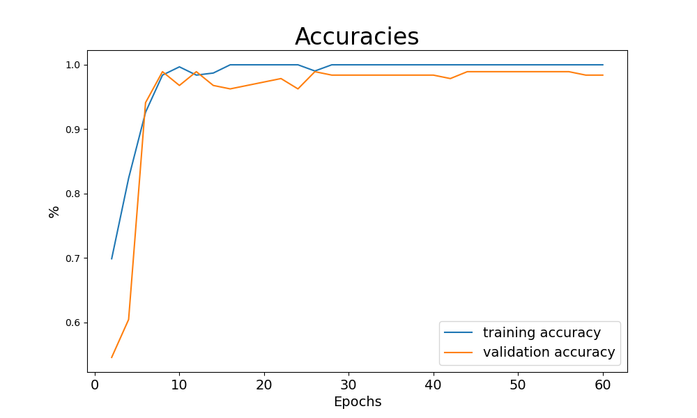
The printouts from training inform that the loss has reduced significantly, and the validation accuracy — the accuracy on data the model has not used for updating its parameters — has reached 98.4%.

An even better impression on the training progress is obtained if we plot the training and validation accuracy over the epochs. We can easily do this because we saved the values each second epoch.
We create a matplotlib figure and axes with plt.subplots() and plot the values over the keys of the accuracy dictionaries.

# Instantiate figure and axe object
fig, ax = plt.subplots(figsize=(10,6))
plt.plot(list(acc_train.keys()), list(acc_train.values()), label="training accuracy")
plt.plot(list(acc_val.keys()), list(acc_val.values()), label="validation accuracy")
plt.title("Accuracies", fontsize=24)
plt.ylabel("%", fontsize=14)
plt.xlabel("Epochs", fontsize=14)
plt.setp(ax.get_xticklabels(), fontsize=14)
plt.legend(loc='best', fontsize=14)
plt.show()

2.13 Loading the trained model

If you want to use the model for production and not only for study purpose, it is highly recommended to save and load the model with all its parameters. Saving was already part of the training code. Loading the model from your drive is equally simple.

# Read model from file
model = torch.load("model.pth")
model.eval()

2.14 Double-check the model accuracy with test data

Remember, we reserved another 20% of our data for testing. This data is totally new to the model and has never been loaded before. We can use this brand-new data to double-check the validation accuracy. Since the validation data has been loaded but never been used to update the model parameters, we expect a similar accuracy to the test value. To conduct the test, we call the val_test() function on the test_loader.

print(f"test accuracy: {val_test(test_loader,model)[0]*100:0.1f}%")

In the specific example, we reach a test accuracy of 99.2%, but this is highly dependent on chance (remember: random distribution of images to training, validation, and testing data).

2.15 Visualizes the misclassified images

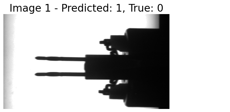
The visualization of the misclassified images is pretty straightforward. First, we call the val_test() function. It returns a tuple with the accuracy value at index position 0 (tup[0]) and another tuple at index position 1 (tup[1]) with the image data (tup[1][0]), the predicted labels (tup[1][1]), and the true labels (tup[1][2]) of the misclassified images. In case tup[1] is not empty, we enumerate it and plot the misclassified images with appropriate headings.

%matplotlib inline

# Call test function
tup = val_test(test_loader, model)

# Check if wrong predictions occur
if len(tup[1])>=1:
    
    # Loop over wrongly predicted images
    for i, t in enumerate(tup[1]):
        plt.figure(figsize=(7,5))
        img, y_pred, y_true = t
        img = img.to("cpu").reshape(400, 700)
        plt.imshow(img, cmap="gray")
        plt.title(f"Image {i+1} - Predicted: {y_pred}, True: {y_true}", fontsize=24)
        plt.axis("off")
        plt.show()
        plt.close()
else:
    print("No wrong predictions!")

In our example, we have only one misclassified image, which represents 0.8% of the test dataset (we have 125 test images). The image was classified as OK but has the label nOK. Frankly, I would have misclassified it too :).

Part 3: Using the trained model in production

3.1 Loading the model, required libraries, and parameters

In the production phase, we assume that the CNN model is trained and the parameters are ready to be loaded. Our aim is to load new images into the model and let it classify whether the respective electronic component is good for assembly or not (see chapter 1.1 The task: Classify an industrial component as good or scrap).

We start by loading the required libraries, setting the device as ‘cuda’ or ‘cpu’, defining the class CNN (exactly as in chapter 2.8), and loading the model from file with torch.load(). We need to define the class CNN before loading the parameters; otherwise, the parameters cannot be assigned correctly.

# Load the required libraries
import torch
import torch.nn as nn
from torch.utils.data import DataLoader, Dataset
from torchvision import datasets, transforms
import matplotlib.pyplot as plt
from PIL import Image
import os

# Device configuration
device = torch.device('cuda' if torch.cuda.is_available() else 'cpu')

# Define the CNN model exactly as in chapter 2.8
class CNN(nn.Module):

    def __init__(self):
        super(CNN, self).__init__()

        # Define model layers
        self.model_layers = nn.Sequential(

            nn.Conv2d(in_channels=1, out_channels=6, kernel_size=5),
            nn.ReLU(),
            nn.MaxPool2d(kernel_size=2, stride=2),

            nn.Conv2d(in_channels=6, out_channels=16, kernel_size=5),
            nn.ReLU(),
            nn.MaxPool2d(kernel_size=2, stride=2),

            nn.Flatten(),
            nn.Linear(16*97*172, 120),
            nn.ReLU(),
            nn.Linear(120, 2),
            #nn.LogSoftmax(dim=1)
        )
        
    def forward(self, x):
        out = self.model_layers(x)
        return out

# Load the model's parameters
model = torch.load("model.pth")
model.eval()

With running this code snippet, we have the CNN model loaded and parameterized in our computer’s memory.

3.2 Load images into dataset

As for the training phase, we need to prepare the images for processing in the CNN model. We load them from a specified folder, crop the inner 700×400 pixels, and transform the image data to a PyTorch tensor.

# Define custom dataset
class Predict_Set(Dataset):
    def __init__(self, img_folder, transform):
        self.img_folder = img_folder
        self.transform = transform
        self.img_lst = os.listdir(self.img_folder)

    def __len__(self):
        return len(self.img_lst)

    def __getitem__(self, idx):
        img_path = os.path.join(self.img_folder, self.img_lst[idx])
        img = Image.open(img_path)
        img = img.crop((50, 60, 750, 460))  #Size: 700x400
        img.load()
        img_tensor = self.transform(img)
        return img_tensor, self.img_lst[idx]

We perform all the steps in a custom dataset class called Predict_Set(). In __init__(), we specify the image folder, accept a transform function, and load the images from the image folder into the list self.img_lst. The method __len__() returns the number of images in the image folder. __getitem__() composes the path to an image from the folder path and the image name, crops the inner part of the image (as we did for the training dataset), and applies the transform function to the image. Finally, it returns the image tensor and the image name.

3.3 Path, transform function, and data loader

The final step in data preparation is to define a data loader that allows to iterate over the images for classification. Along the way, we specify the path to the image folder and define the transform function as a pipeline that first loads the image data to a PyTorch tensor, and, second, normalizes the data to a range of approximately -1 to +1. We instantiate our custom dataset Predict_Set() to a variable predict_set and define the data loader predict_loader. Since we do not specify a batch size, predict_loader returns one image at a time.

# Path to images (preferably local to accelerate loading)
path = "data/Coil_Vision/02_predict"

# Transform function for loading
transform = transforms.Compose([transforms.ToTensor(),
                                transforms.Normalize((0.5), (0.5))])

# Create dataset as instance of custom dataset
predict_set = Predict_Set(path, transform=transform)

# Define loader
predict_loader = DataLoader(dataset=predict_set)

3.4 Custom function for classification

So far, the preparation of the image data for classification is complete. However, what we are still missing is a custom function that transfers the images to the CNN model, translates the model’s response into a classification, and returns the classification results. This is exactly what we do with predict().

def predict(dataloader, model):

    # Turn off gradient calculation
    with torch.no_grad():
        
        img_lst = []; y_pred_lst = []; name_lst = []
        # Loop over data loader
        for image, name in dataloader:
            img_lst.append(image)
            image = image.to(device)
            
            # Get raw values from model
            output = model(image)
            
            # Derive prediction
            y_pred = output.argmax(1)
            y_pred_lst.append(y_pred.item())
            name_lst.append(name[0])
            
    return img_lst, y_pred_lst, name_lst

predict() expects a data loader and the CNN model as its parameters. In its core, it iterates over the data loader, transfers the image data to the model, and interprets the models response with output.argmax(1) as the classification result — either 0 for scrap parts (nOK) or 1 for good parts (OK). The image data, the classification result, and the image name are appended to lists and the lists are returned as the function’s result.

3.5 Predict labels and plot images

Finally, we want to utilize our custom functions and loaders to classify new images. In the folder “data/Coil_Vision/02_predict” we have reserved four images of electronic components that wait to be inspected. Remember, we want the CNN model to tell us whether we can use the components for automatic assembly or if we need to sort them out because the pins are likely to cause problems while trying to push them in the plug sockets.
We call the custom function predict(), which returns a list of images, a list of classification results, and a list of image names. We enumerate the lists and plot the images with the names and the classification as headings.

# Predict labels for images
imgs, lbls, names  = predict(predict_loader, model)

# Iterate over classified images
for idx, image in enumerate(imgs):
    plt.figure(figsize=(8,6))
    plt.imshow(image.squeeze(), cmap="gray")
    plt.title(f"nFile: {names[idx]}, Predicted label: {lbls[idx]}", fontsize=18)
    plt.axis("off")
    plt.show()
    plt.close()

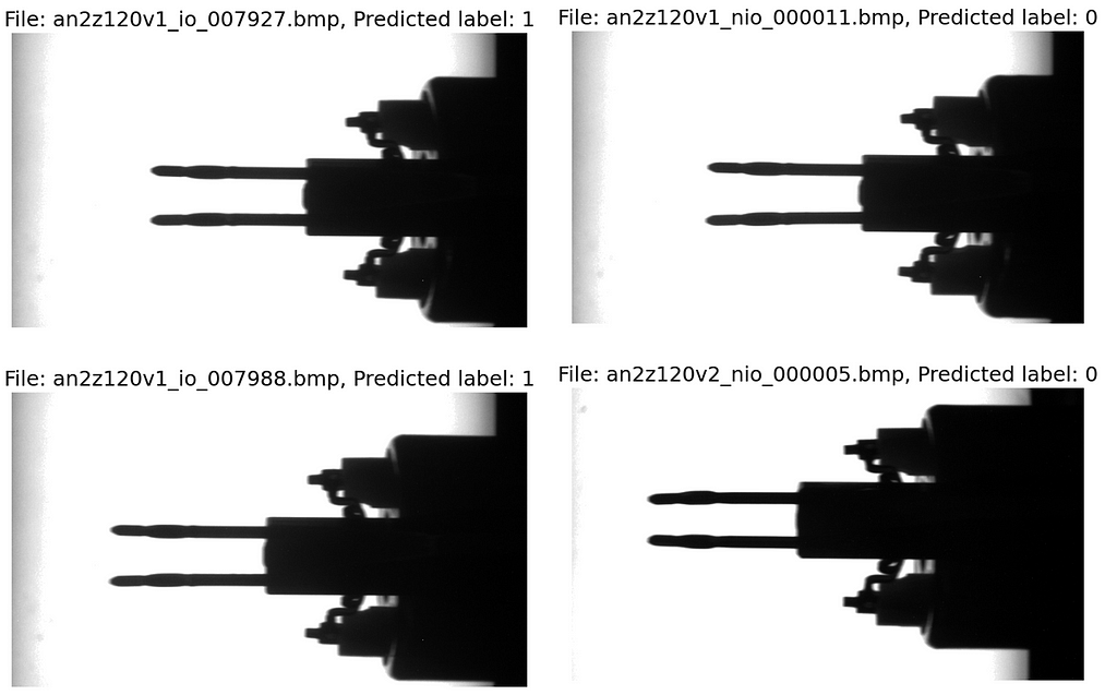
We see that the two images on the left side have been classified a good (label 1) and the two on the right as scrap (label 0). Due to our training data, the model is quite sensitive, and even small bends in the pins lead to them being classified as scrap.

Part 4: What did the CNN consider in its “decision”?

We have gone deep into the details of the CNN and our industrial use case so far. This seems like a good opportunity to take one step further and try to understand what the CNN model “sees” while processing the image data. To do this, we first study the convolutional layers and then examine which parts of the image are specifically important for the classification.

4.1 Study the convolutional filters’ dimensions

To gain a better understanding of how convolutional filters work and what they do to the images, let’s examine the layers in our industrial example in more detail.

To access the layers, we enumerate model.children(), which is a generator for the model’s structure. If the layer is a convolutional layer, we append it to the list all_layers and save the weights’ dimensions in conv_weights. If we have a ReLU or a MaxPooling layer, we have no weights. In this case, we append the layer and “*” to the respective lists. Next, we enumerate all_layers, print the layer type, and the weights’ dimensions.

# Empty lists to store the layers and the weights
all_layers = []; conv_weights = []

# Iterate over the model's structure
# (First level nn.Sequential)
for _, layer in enumerate(list(model.children())[0]):
    if type(layer) == nn.Conv2d:
        all_layers.append(layer)
        conv_weights.append(layer.weight)
    elif type(layer) in [nn.ReLU, nn.MaxPool2d]:
        all_layers.append(layer)
        conv_weights.append("*")

# Print layers and dimensions of weights
for idx, layer in enumerate(all_layers):
    print(f"{idx+1}. Layer: {layer}")
    if type(layer) == nn.Conv2d:
        print(f"          weights: {conv_weights[idx].shape}")
    else:
        print(f"          weights: {conv_weights[idx]}")
    print()

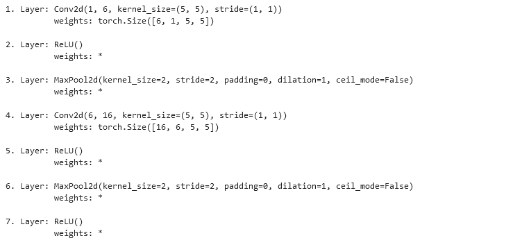
Please compare the code snippet’s output with Fig. 3. The first convolutional layer has one input — the original image with only one channel — and returns six feature maps. We apply six kernels, each of depth one and size 5×5. Correspondingly, the weights are of dimension torch.Size([6, 1, 5, 5]). In contrast, layer 4 receives six feature maps as input and returns 16 maps as output. We apply 16 convolutional kernels, each of depth 6 and size 5×5. The weights’ dimension is therefore torch.Size([16, 6, 5, 5]).

4.2 Visualize the convolutional filters’ weights

Now, we know the convolutional filters’ dimensions. Next, we want to see their weights, which they have gained during the training process. Since we have so many different filters (six in the first convolutional layer and 16 in the second), we select, in both cases, the first input channel (index 0).

import itertools

# Iterate through all layers
for idx_out, layer in enumerate(all_layers):
    
    # If layer is a convolutional filter
    if type(layer) == nn.Conv2d:
        
        # Print layer name
        print(f"n{idx_out+1}. Layer: {layer} n")
        
        # Prepare plot and weights
        plt.figure(figsize=(25,6))
        weights = conv_weights[idx_out][:,0,:,:] # only first input channel
        weights = weights.detach().to('cpu')
        
        # Enumerate over filter weights (only first input channel)
        for idx_in, f in enumerate(weights):
            plt.subplot(2,8, idx_in+1)
            plt.imshow(f, cmap="gray")
            plt.title(f"Filter {idx_in+1}")
            
            # Print texts
            for i, j in itertools.product(range(f.shape[0]), range(f.shape[1])):
                if f[i,j] > f.mean():
                    color = 'black'
                else:
                    color = 'white'
                plt.text(j, i, format(f[i, j], '.2f'), horizontalalignment='center', verticalalignment='center', color=color)
            
            plt.axis("off")
        plt.show()
        plt.close()       

We iterate over all_layers. If the layer is a convolutional layer (nn.Conv2d), then we print the layer’s index and the layer’s core data. Next, we prepare a plot and extract the weights matrix for the first input layer as an example. We enumerate all output layers and plot them with plt.imshow(). Finally, we print the weights’ values on the image so that we get an intuitive visualization of the convolutional filters.

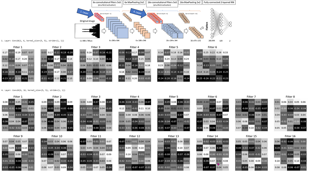
Fig. 12 shows the six convolutional filter kernels of layer 1 and the 16 kernels of layer 4 (for input channel 0). The model schematic in the upper right indicates the filters with a red outline. We see that the majority of values are close to 0, and some are in the range of positive or negative 0.20–0.25. The numbers represent the values used for the convolution demonstrated in Fig. 4. This gives us the feature maps, which we inspect next.

4.3 Examine the feature maps

According to Fig. 4, we receive the first feature maps through the convolution of the input image. Therefore, we load a random image from the test_loader and push it to the CPU (in case you operate the CNN on the GPU).

# Test loader has a batch size of 1
img = next(iter(test_loader))[0].to(device)
print(f"nImage has shape: {img.shape}n")

# Plot image
img_copy = img.to('cpu')
plt.imshow(img_copy.reshape(400,700), cmap="gray")
plt.axis("off")
plt.show()

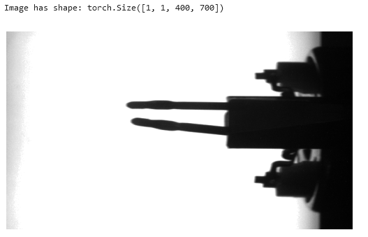
Now we pass the image data img through the first convolution layer (all_layers[0]) and save the output in results. Next, we iterate over all_layers and feed the next layer with the output from the previous layer operation. Those operations are convolutions, ReLU activations or MaxPoolings. The output of each operation we append to results.

# Pass the image through the first layer
results = [all_layers[0](img)]

# Pass the results of the previous layer to the next layer
for idx in range(1, len(all_layers)):  # Start at 1, first layer already passed!
    results.append(all_layers[idx](results[-1]))  # Pass the last result to the layer

Finally, we plot the original image, the feature maps after passing the first layer (convolution), the second layer (ReLU), the third layer (MaxPooling), the forth layer (2nd convolution), the fifth layer (2nd ReLU), and the sixth layer (2nd MaxPooling).

We see that the convolutional kernels (compare Fig. 12) recalculate each pixel of the image. This appears as changed grayscale values in the feature maps. Some of the feature maps are sharpened compared to the original image or have a stronger black-and-white contrast, while others seem to be faded.

The ReLU operations turn dark gray into black since negative values are set to zero.

MaxPooling keeps the images almost unchanged while halving the image size in both dimensions.

4.4 Visualize the image areas that impact the classification the most

Before we finish, let’s analyze which areas of the image are particularly decisive for the classification into scrap (index 0) or good parts (index 1). For this purpose, we use Gradient-weighted Class Activation Mapping (gradCAM). This technique computes the gradients of the trained model with respect to the predicted class (the gradients show how much the inputs — the image pixels — influence the prediction). The averages of the gradients of each feature map (= output channel of convolution layer) build the weights with which the feature maps are multiplied when calculating a heat map for visualization.
But let’s look at one step after the other.

def gradCAM(x):
    
    # Run model and predict
    logits = model(x)
    pred = logits.max(-1)[-1] # Returns index of max value (0 or 1)
    
    # Fetch activations at final conv layer
    last_conv = model.model_layers[:5]
    activations = last_conv(x)

    # Compute gradients with respect to model's prediction
    model.zero_grad()
    logits[0,pred].backward(retain_graph=True)
    
    # Compute average gradient per output channel of last conv layer
    pooled_grads = model.model_layers[3].weight.grad.mean((1,2,3))
    
    # Multiply each output channel with its corresponding average gradient
    for i in range(activations.shape[1]):
        activations[:,i,:,:] *= pooled_grads[i]
    
    # Compute heatmap as average over all weighted output channels
    heatmap = torch.mean(activations, dim=1)[0].cpu().detach()
    
    return heatmap

We define a function gradCAM that expects the input data x, an image or a feature map, and returns a heatmap.

In the first block, we input x in the CNN model and receive logits, a tensor of shape [1, 2] with two values only. The values represent the predicted probabilities of the classes 0 and 1. We select the index of the larger value as the model’s prediction pred.

In the second block, we extract the first five layers of the model — from first convolution to second ReLU — and save them to last_conv. We run x through the selected layers and store the output in activations. As the name suggests, those are the activations (=feature maps) of the second convolutional layer (after ReLU activation).

In the third block, we do the backward propagation for the logit value of the predicted class logits[0,pred]. In other words, we compute all the gradients of the CNN with respect to the prediction. The gradients show how much a change in the input data — the original image pixels — impact the models output — the prediction. The result is saved in the PyTorch computational graph until we delete it with model.zero_grad().

In the fourth block, we compute the averages of the gradients over the input channel, as well as the height and width of the image or the feature maps. As a result, we receive 16 average gradients for the 16 feature maps that are returned from the second convolutional layer. We save them in pooled_grads.

In the fifth block, we iterate over the 16 feature maps returned from the second convolutional layer and weight them with the average gradients pooled_grads. This operation gives more impact to those feature maps (and their pixels) that have high importance for the prediction and vice versa. From now on, activations holds not the feature maps, but the weighted feature maps.

Finally, in the last block, we compute the heatmap as the average feature map of all activations. This is what the function gradCAM returns.

Before we can plot the image and the heatmap, we need to transform both for the overlay. Remember, the feature maps are smaller than the original picture (see chapters 1.3 and 1.7), and so is the heatmap. This is why we need the function upsampleHeatmap(). The function scales the pixel values to the range of 0 to 255 and transforms them to 8-bit integer format (required from the cv2 library). It resizes the heatmap to 400×700 px and applies a color map to both the image and heatmap. Finally, we overlay 70% heatmap and 30% image and return the composition for plotting.

import cv2

def upsampleHeatmap(map, img):
    m,M = map.min(), map.max()
    i,I = img.min(), img.max()
    map = 255 * ((map-m) / (M-m))
    img = 255 * ((img-i) / (I-i))
    map = np.uint8(map)
    img = np.uint8(img)
    map = cv2.resize(map, (700,400))
    map = cv2.applyColorMap(255-map, cv2.COLORMAP_JET)
    map = np.uint8(map)
    img = cv2.applyColorMap(255-img, cv2.COLORMAP_JET)
    img = np.uint8(img)
    map = np.uint8(map*0.7 + img*0.3)
    return map

We want to plot the original image and the heatmap overlay next to each other in one row. To do this, we iterate over the data loader predict_loader, run the gradCAM() function on the images and the upsampleHeatmap() function on the heatmap and the image. Finally, we plot the original image and the heatmap in a row with matplotlib.pyplot.

# Iterate over dataloader
for idx, (image, name) in enumerate(predict_loader):
    
    # Compute heatmap
    image = image.to(device)
    heatmap = gradCAM(image)
    image = image.cpu().squeeze(0).permute(1,2,0)
    heatmap = upsampleHeatmap(heatmap, image)
    
    # Plot images and heatmaps
    fig = plt.figure(figsize=(14,5))
    fig.suptitle(f"nFile: {names[idx]}, Predicted label: {lbls[idx]}n", fontsize=24)
    plt.subplot(1, 2, 1)
    plt.imshow(image, cmap="gray")
    plt.title(f"Image", fontsize=14)
    plt.axis("off")
    plt.subplot(1, 2, 2)
    plt.imshow(heatmap)
    plt.title(f"Heatmap", fontsize=14)
    plt.tight_layout()
    plt.axis("off")
    plt.show()
    plt.close()

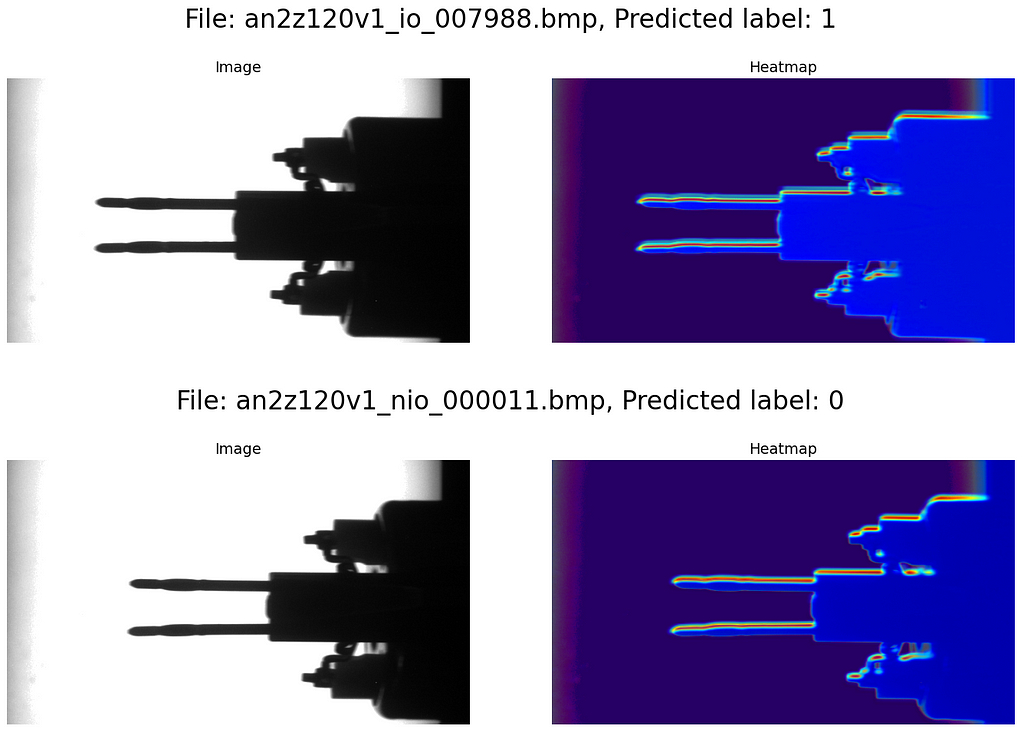
The blue areas of the heatmap have low impact on the model’s decision, while the yellow and red areas are very important. We see that in our use case, mainly the contour of the electronic component (in particular the metal pins) is decisive for the classification into scrap or good parts. Of course, this is highly reasonable, given that the use case primarily deals with bent pins.

Conclusion

Convolutional Neural Networks (CNNs) are nowadays a common and widely used tool for visual inspection tasks in the industrial environment. In our use case, with relatively few lines of code, we managed to define a model that classifies electronic components as good parts or scrap with high precision. The big advantage, compared to classic approaches of vision inspection, is that no process engineer needs to specify visual marks in the images for the classification. Instead, the CNN learns from labeled examples and is able to replicate this knowledge to other images. In our specific use case, 626 labeled images were sufficient for training and validation. In more complex cases, the demand for training data might be significantly higher.

Algorithms like gradCAM (Gradient-weighted Class Activation Mapping) significantly help in understanding which areas in the image are particularly relevant for the model’s decision. In this way, they support a broad use of CNNs in the industrial context by building trust in the model’s functionality.

In this article, we have explored many details of the inner workings of Convolutional Neural Networks. I hope you enjoyed the journey and have gained a deep understanding of how CNNs work.

Building a Vision Inspection CNN for an Industrial Application was originally published in Towards Data Science on Medium, where people are continuing the conversation by highlighting and responding to this story.