Quantizing the Weights of AI Models

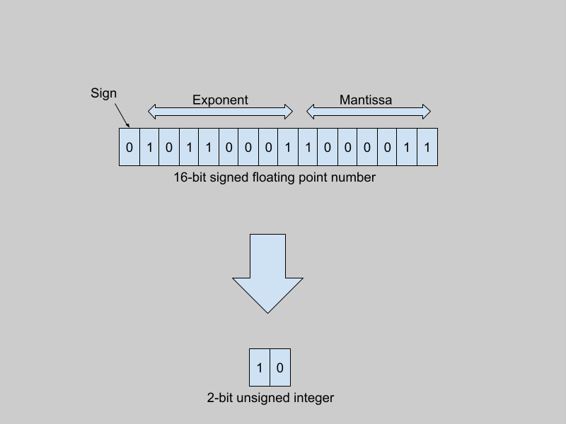
Reducing high-precision floating-point weights to low-precision integer weights

To make AI models more affordable and accessible, many developers and researchers are working towards making the models smaller but equally powerful. Earlier in this series, the article Reducing the Size of AI Models gives a basic introduction to quantization as a successful technique to reduce the size of AI models. Before learning more about the quantization of AI models, it is necessary to understand how the quantization operation works.

This article, the second in the series, presents a hands-on introduction to the arithmetics of quantization. It starts with a simple example of scaling number ranges and progresses to examples with clipping, rounding, and different types of scaling factors.

There are different ways to represent real numbers in computer systems, such as 32-bit floating point numbers, 8-bit integers, and so on. Regardless of the representation, computers can only express numbers in a finite range and of a limited precision. 32-bit floating point numbers (using the IEEE 754 32-bit base-2 system) have a range from -3.4 * 10³⁸ to +3.4 * 10³⁸. The smallest positive number that can be encoded in this format is of the order of 1 * 10^-38. In contrast, signed 8-bit integers range from -128 to +127.

Traditionally, model weights are represented as 32-bit floats (or as 16-bit floats, in the case of many large models). When quantized to 8-bit integers (for example), the quantizer function maps the entire range of 32-bit floating point numbers to integers between -128 and +127.

Scaling Number Ranges

Consider a rudimentary example: you need to map numbers in the integer range A from -1000 to 1000 to the integer range B from -10 to +10. Intuitively, the number 500 in range A maps to the number 5 in range B. The steps below illustrate how to do this formulaically:

• To transform a number from one range to another, you need to multiply it by the right scaling factor. The number 500 from range A can be expressed in the range B as follows:

500 * scaling_factor = Representation of 500 in Range B = 5

• To calculate the scaling factor, take the ratio of the difference between the maximum and minimum values of the target range to the original range:

• To map the number 500, multiply it by the scaling factor:

500 * (1/100) = 5

• Based on the above formulation, try to map the number 510:

510 * (1/100) = 5.1

• Since the range B consists only of integers, extend the above formula with a rounding function:

Round ( 510 * (1/100) ) = 5

• Similarly, all the numbers from 500 to 550 in Range A map to the number 5 in Range B. Based on this, notice that the mapping function resembles a step function with uniform steps.

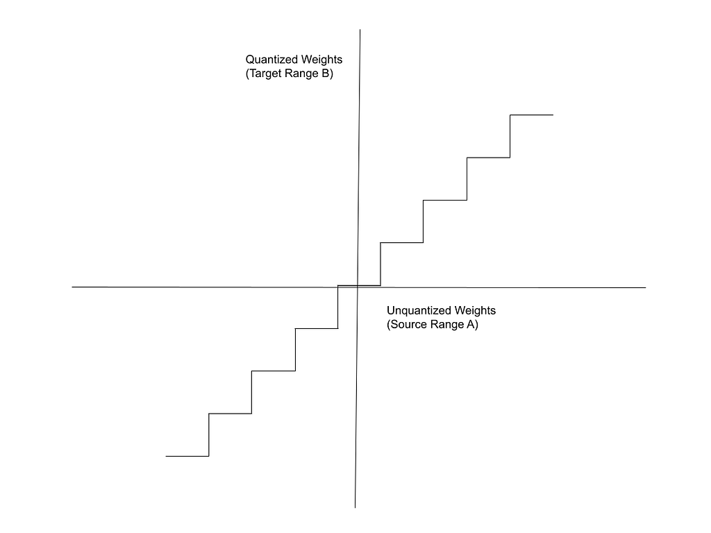
The X-axis in this figure represents the source Range, A (unquantized weights) and the Y-axis represents the target Range, B (quantized weights).

Simple Integer Quantization

As a more practical example, consider a floating point range -W to +W, which you want to quantize to signed N-bit integers. The range of signed N-bit integers is -2^(N-1) to +2^(N-1)-1. But, to simplify things for the sake of illustration, assume a range from -2^(N-1) to +2^(N-1). For example, (signed) 8-bit integers range from -16 to +15 but here we assume a range from -16 to +16. This range is symmetric around 0 and the technique is called symmetric range mapping.

• The scaling factor, s, is:

• The quantized number is the product of the unquantized number and the scaling factor. To quantize to integers, we need to round this product to the nearest integer:

To remove the assumption that the target range is symmetric around 0, you also account for the zero-point offset, as explained in the next section.

Zero Point Quantization

The number range -2^(N-1) to +2^(N-1), used in the previous example, is symmetric around 0. The range -2^(N-1) to +2^(N-1)-1, represented by N-bit integers, is not symmetric.

When the quantization number range is not symmetric, you add a correction, called a zero point offset, to the product of the weight and the scaling factor. This offset shifts the range such that it is effectively symmetric around zero. Conversely, the offset represents the quantized value of the number 0 in the unquantized range. The steps below show how to calculate the zero point offset, z.

• The quantization relation with the offset is expressed as:

• Map the extreme points of the original and the quantized intervals. In this context, W_min and W_max refer to the minimum and maximum weights in the original unquantized range.

• Solving these linear equations for the scaling factor, s, we get:

• Similarly, we can express the offset, z, in terms of scaling factor s, as:

• Substituting for s in the above relation:

• Since we are converting from floats to integers, the offset also needs to be an integer. Rounding the above expression:

Meaning of Zero-Point

In the above discussion, the offset value is called the zero-point offset. It is called the zero-point because it is the quantized value of the floating point weight of 0.

When W = 0 in

You get:

The article, Zero-point quantization: How do we get those formulas, by Luis Vasquez, discusses zero-point quantization with many examples and illustrative pictures.

De-quantization

The function to obtain an approximation of the original floating point value from the quantized value is called the de-quantization function. It is simply the inverse of the original quantization relation:

Ideally, the de-quantized weight should be equal to the original weight. But, because of the rounding operations in the quantization functions, this is not the case. Thus, there is a loss of information involved in the de-quantization process.

Improving the Precision of Quantization

The biggest drawback of the above methods is the loss of precision. Bhandare et al, in a 2019 paper titled Efficient 8-Bit Quantization of Transformer Neural Machine Language Translation Model, were the first to quantize Transformer models. They demonstrated that naive quantization, as discussed in earlier sections, results in a loss of precision. In gradient descent, or indeed any optimization algorithm, the weights undergo just a slight modification in each pass. It is therefore important for the quantization method to be able to capture fractional changes in the weights.

Clipping the Range

Quantized intervals have a fixed and limited range of integers. On the other hand, unquantized floating points have a very large range. To increase the precision, it is helpful to reduce (clip) the range of the floating point interval.

It is observed that the weights in a neural network follow a statistical distribution, such as a normal Gaussian distribution. This means, most of the weights fall within a narrow interval, say between W_max and W_min. Beyond W_max and W_min, there are only a few outliers.

In the following description, the weights are clipped, and W_max and W_min refer to the maximum and minimum values of the weights in the clipped range.

Clipping (restricting) the range of the floating point weights to this interval means:

• Weights which fall in the tails of the distribution are clipped — Weights higher than W_max are clipped to W_max. Weights smaller than W_min are clipped to W_min. The range between W_min and W_max is the clipping range.
• Because the range of the floating point weights is reduced, a smaller unquantized range maps to the same quantized range. Thus, the quantized range can now account for smaller changes in the values of the unquantized weights.

The quantization formula shown in the previous section is modified to include the clipping:

The clipping range is customizable. You can choose how narrow you want this interval to be. If the clipping is overly aggressive, weights that contribute to the model’s accuracy can be lost in the clipping process. Thus, there is a tradeoff — clipping to a very narrow interval increases the precision of the quantization of weights within the interval, but it also reduces the model’s accuracy due to loss of information from those weights which were considered as outliers and got clipped.

Determining the Clipping Parameters

It has been noted by many researchers that the statistical distribution of model weights has a significant effect on the model’s performance. Thus, it is essential to quantize weights in such a way that these statistical properties are preserved through the quantization. Using statistical methods, such as Kullback Leibler Divergence, it is possible to measure the similarity of the distribution of weights in the quantized and unquantized distributions.

The optimal clipped values of W_max and W_min are chosen by iteratively trying different values and measuring the difference between the histograms of the quantized and unquantized weights. This is called calibrating the quantization. Other approaches include minimizing the mean square error between the quantized weights and the full-precision weights.

Different Scaling Factors

There is more than one way to scale floating point numbers to lower precision integers. There are no hard rules on what is the right scaling factor. Researchers have experimented with various approaches. A general guideline is to choose a scaling factor so that the unquantized and quantized distributions have a similar statistical properties.

MinMax Quantization

The examples in the previous sections scale each weight by the difference of W_max and W_min (the maximum and minimum weights in the set). This is known as minmax quantization.

This is one of the most common approaches to quantization.

AbsMax Quantization

It is also possible to scale the weights by the absolute value of the maximum weight:

Wang et al, in their 2023 paper titled BitNet: Scaling 1-bit Transformers for Large Language Models, use absmax quantization to build the 1-bit BitNet Transformer architecture. The BitNet architecture is explained later in this series, in Understanding 1-bit Large Language Models.

AbsMean Quantization

Another approach is to make the scaling factor equal to the average of the absolute values of all the unquantized weights:

Ma et al, in the 2024 paper titled The Era of 1-bit LLMs: All Large Language Models are in 1.58 Bits, use absmean quantization to build a 1.58-bit variant of BitNet. To learn more about 1.58-bit language models, refer to Understanding 1.58-bit Large Language Models.

Granularity of Quantization

It is possible to quantize all the weights in a model using the same quantization scale. However, for better accuracy, it is also common to calibrate and estimate the range and quantization formula separately for each tensor, channel, and layer. The article Different Approaches to Quantization discusses the granularity levels at which quantization is applied.

Extreme Quantization

Traditional quantization approaches reduce the precision of model weights to 16-bit or 8-bit integers. Extreme quantization refers to quantizing weights to 1-bit and 2-bit integers. Quantization to 1-bit integers ({0, 1}) is called binarization. The simple approach to binarize floating point weights is to map positive weights to +1 and negative weights to -1:

Similarly, it is also possible to quantize weights to ternary ({-1, 0, +1}):

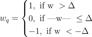
In the above system, Delta is a threshold value. In a simplistic approach, one might quantize to ternary as follows:

• Normalize the unquantized weights to lie between -1 and +1
• Quantize weights below -0.5 to -1
• Quantize weights between -0.5 and +0.5 to 0
• Quantize weights above 0.5 to +1.

Directly applying binary and ternary quantization leads to poor results. As discussed earlier, the quantization process must preserve the statistical properties of the distribution of the model weights. In practice, it is common to adjust the range of the raw weights before applying the quantization and to experiment with different scaling factors.

Later in this series, the articles Understanding 1-bit Large Language Models and Understanding 1.58-bit Language Models discuss practical examples of binarization and ternarization of weights. The 2017 paper titled Trained Ternary Quantization by Zhu et al and the 2023 survey paper on ternary quantization by Liu et al dive deeper into the details of ternary quantization.

The premise of binarization is that even though this process (binarization) seems to result in a loss of information, using a large number of weights compensates for this loss. The statistical distribution of the binarized weights is similar to that of the unquantized weights. Thus, deep neural networks are still able to demonstrate good performance even with binary weights.

Non-uniform Quantization

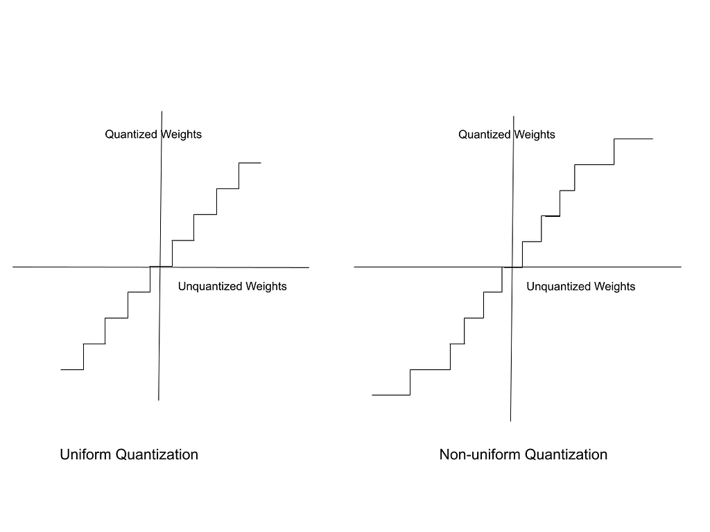
The quantization methods discussed so far uniformly map the range of unquantized weights to quantized weights. They are called “uniform” because the mapping intervals are equidistant. To clarify, when you mapped the range -1000 to +1000 to the range -10 to +10:

• All the numbers from -1000 to -951 are mapped to -10
• The interval from -950 to -851 is mapped to -9
• The interval from -850 to -751 maps to -8
• and so on…

These intervals are also called bins.

The disadvantage of uniform quantization is that it does not take into consideration the statistical distribution of the weights themselves. It works best when the weights are equally distributed between W_max and W_min. The range of floating point weights can be considered as divided into uniform bins. Each bin maps to one quantized weight.

In reality, floating point weights are not distributed uniformly. Some bins contain a large number of unquantized weights while other bins have very few. Non-uniform quantization aims to create these bins in such a way that bins with a higher density of weights map to a larger interval of quantized weights.

There are different ways of representing the non-uniform distribution of weights, such as K-means clustering. However, these methods are not currently used in practice, due to the computational complexity of their implementation. Most practical quantization systems are based on uniform quantization.

In the hypothetical graph below, in the chart on the right, unquantized weights have a low density of distribution towards the edges and a high density around the middle of the range. Thus, the quantized intervals are larger towards the edges and compact in the middle.

Quantizing Activations and Biases

The activation is quantized similarly as the weights are, but using a different scale. In some cases, the activation is quantized to a higher precision than the weights. In models like BinaryBERT, and the 1-bit Transformer — BitNet, the weights are quantized to binary but the activations are in 8-bit.

The biases are not always quantized. Since the bias term only undergoes a simple addition operation (as opposed to matrix multiplication), the computational advantage of quantizing the bias is not significant. Also, the number of bias terms is much less than the number of weights.

Conclusion

This article explained (with numerical examples) different commonly used ways of quantizing floating point model weights. The mathematical relationships discussed here form the foundation of quantization to 1-bit weights and to 1.58-bit weights — these topics are discussed later in the series.

To learn more about the mathematical principles of quantization, refer to this 2023 survey paper by Weng. Quantization for Neural Networks by Lei Mao explains in greater detail the mathematical relations involved in quantized neural networks, including non-linear activation functions like the ReLU. It also has code samples implementing quantization. The next article in this series, Quantizing Neural Network Models, presents the high-level processes by which neural network models are quantized.

Quantizing the Weights of AI Models was originally published in Towards Data Science on Medium, where people are continuing the conversation by highlighting and responding to this story.