Dynamic Execution

Getting your AI task to distinguish between Hard and Easy problems

In this position paper, I discuss the premise that a lot of potential performance enhancement is left on the table because we don’t often address the potential of dynamic execution.

I guess I need to first define what is dynamic execution in this context. As many of you are no doubt aware of, we often address performance optimizations by taking a good look at the model itself and what can be done to make processing of this model more efficient (which can be measured in terms of lower latency, higher throughput and/or energy savings).

These methods often address the size of the model, so we look for ways to compress the model. If the model is smaller, then memory footprint and bandwidth requirements are improved. Some methods also address sparsity within the model, thus avoiding inconsequential calculations.

Still… we are only looking at the model itself.

This is definitely something we want to do, but are there additional opportunities we can leverage to boost performance even more? Often, we overlook the most human-intuitive methods that don’t focus on the model size.

Hard vs Easy

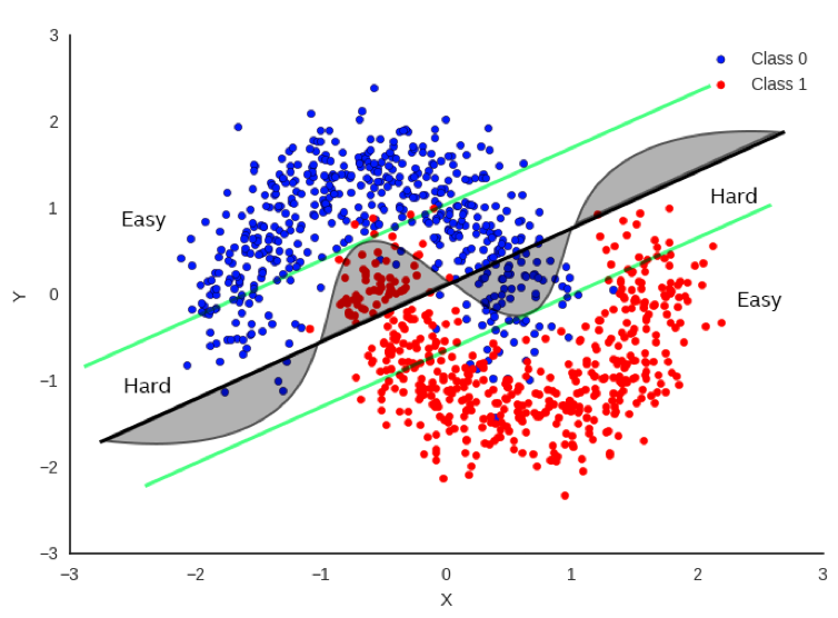
In Figure 1, there’s a simple example (perhaps a bit simplistic) regarding how to classify between red and blue data points. It would be really useful to be able to draw a decision boundary so that we know the red and blue points are on opposite sides of the boundary as much as possible. One method is to do a linear regression whereby we fit a straight line as best as we can to separate the data points as much as possible. The bold black line in Figure 1 represents one potential boundary. Focusing only on the bold black line, you can see that there is a substantial number of points that fall on the wrong side of the boundary, but it does a decent job most of the time.

If we focus on the curved line, this does a much better job, but it’s also more difficult to compute as it’s no longer a simple, linear equation. If we want more accuracy, clearly the curve is a much better decision boundary than the black line.

But let’s not just throw out the black line just yet. Now let’s look at the green parallel lines on each side of the black boundary. Note that the linear decision boundary is very accurate for points outside of the green line. Let’s call these points “Easy”.

In fact, it is 100% as accurate as the curved boundary for Easy points. Points that lie inside the green lines are “Hard” and there is a clear advantage to using the more complex decision boundary for these points.

So… if we can tell if the input data is hard or easy, we can apply different methods to solving the problem with no loss of accuracy and a clear savings of computations for the easy points.

This is very intuitive as this is exactly how humans address problems. If we perceive a problem as easy, we often don’t think too hard about it and give an answer quickly. If we perceive a problem as being hard, we think more about it and often it takes more time to get to the answer.

So, can we apply a similar approach to AI?

Dynamic Execution Methods

In the dynamic execution scenario, we employ a set of specialized techniques designed to scrutinize the specific query at hand. These techniques involve a thorough examination of the query’s structure, content, and context with the aim of discerning whether the problem it represents can be addressed in a more straightforward manner.

This approach mirrors the way humans tackle problem-solving. Just as we, as humans, are often able to identify problems that are ’easy’ or ’simple’ and solve them with less effort compared to ’hard’ or ’complex’ problems, these techniques strive to do the same. They are designed to recognize simpler problems and solve them more efficiently, thereby saving computational resources and time.

This is why we refer to these techniques as Dynamic Execution. The term ’dynamic’ signifies the adaptability and flexibility of this approach. Unlike static methods that rigidly adhere to a predetermined path regardless of the problem’s nature, Dynamic Execution adjusts its strategy based on the specific problem it encounters, that is, the opportunity is data dependent.

The goal of Dynamic Execution is not to optimize the model itself, but to optimize the compute flow. In other words, it seeks to streamline the process through which the model interacts with the data. By tailoring the compute flow to the data presented to the model, Dynamic Execution ensures that the model’s computational resources are utilized in the most efficient manner possible.

In essence, Dynamic Execution is about making the problem-solving process as efficient and effective as possible by adapting the strategy to the problem at hand, much like how humans approach problem-solving. It is about working smarter, not harder. This approach not only saves computational resources but also improves the speed and accuracy of the problem-solving process.

Early Exit

This technique involves adding exits at various stages in a deep neural network (DNN). The idea is to allow the network to terminate the inference process earlier for simpler tasks, thus saving computational resources. It takes advantage of the observation that some test examples can be easier to predict than others [1], [2].

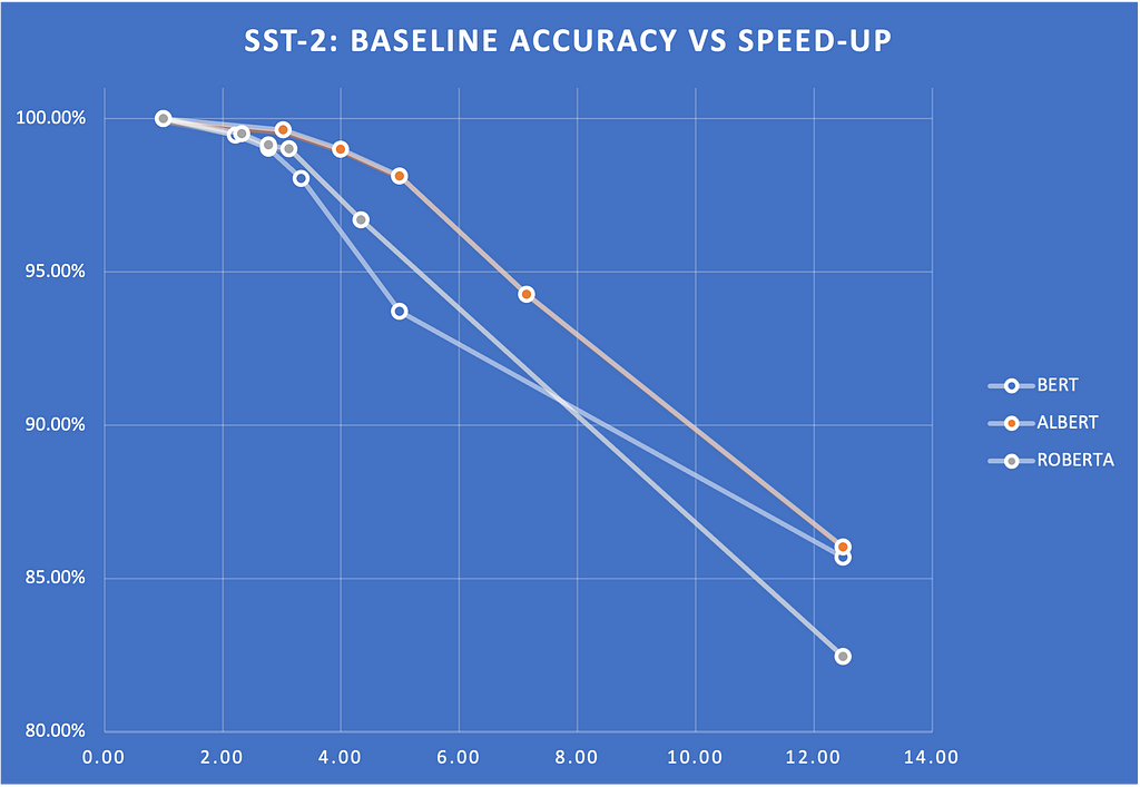
Below is an example of the Early Exit strategy in several encoder models, including BERT, ROBERTA, and ALBERT.

We measured the speed-ups on glue scores for various entropy thresholds. Figure 2 shows a plot of these scores and how they drop with respect to the entropy threshold. The scores show the percentage of the baseline score (that is, without Early Exit). Note that we can get 2x to 4X speed-up without sacrificing much quality.

Speculative Sampling

This method aims to speed up the inference process by computing several candidate tokens from a smaller draft model. These candidate tokens are then evaluated in parallel in the full target model [3], [4].

Speculative sampling is a technique designed to accelerate the decoding process of large language models [5], [6]. The concept behind speculative sampling is based on the observation that the latency of parallel scoring of short continuations, generated by a faster but less powerful draft model, is comparable to that of sampling a single token from the larger target model. This approach allows multiple tokens to be generated from each transformer call, increasing the speed of the decoding process.

The process of speculative sampling involves two models: a smaller, faster draft model and a larger, slower target model. The draft model speculates what the output is several steps into the future, while the target model determines how many of those tokens we should accept. The draft model decodes several tokens in a regular autoregressive fashion, and the probability outputs of the target and the draft models on the new predicted sequence are compared. Based on some rejection criteria, it is determined how many of the speculated tokens we want to keep. If a token is rejected, it is resampled using a combination of the two distributions, and no more tokens are accepted. If all speculated tokens are accepted, an additional final token can be sampled from the target model probability output.

In terms of performance boost, speculative sampling has shown significant improvements. For instance, it was benchmarked with Chinchilla, a 70 billion parameter language model, achieving a 2–2.5x decoding speedup in a distributed setup, without compromising the sample quality or making modifications to the model itself. Another example is the application of speculative decoding to Whisper, a general purpose speech transcription model, which resulted in a 2x speed-up in inference throughput [7], [8]. Note that speculative sampling can be used to boost CPU inference performance, but the boost will likely be less (typically around 1.5x).

In conclusion, speculative sampling is a promising technique that leverages the strengths of both a draft and a target model to accelerate the decoding process of large language models. It offers a significant performance boost, making it a valuable tool in the field of natural language processing. However, it is important to note that the actual performance boost can vary depending on the specific models and setup used.

StepSaver

This is a method that could also be called Early Stopping for Diffusion Generation, using an innovative NLP model specifically fine-tuned to determine the minimal number of denoising steps required for any given text prompt. This advanced model serves as a real-time tool that recommends the ideal number of denoising steps for generating high-quality images efficiently. It is designed to work seamlessly with the Diffusion model, ensuring that images are produced with superior quality in the shortest possible time. [9]

Diffusion models iteratively enhance a random noise signal until it closely resembles the target data distribution [10]. When generating visual content such as images or videos, diffusion models have demonstrated significant realism [11]. For example, video diffusion models and SinFusion represent instances of diffusion models utilized in video synthesis [12][13]. More recently, there has been growing attention towards models like OpenAI’s Sora; however, this model is currently not publicly available due to its proprietary nature.

Performance in diffusion models involves a large number of iterations to recover images or videos from Gaussian noise [14]. This process is called denoising and is trained on a specific number of iterations of denoising. The number of iterations in this sampling procedure is a key factor in the quality of the generated data, as measured by metrics, such as FID.

Latent space diffusion inference uses iterations in feature space, and performance suffers from the expense of many iterations required for quality output. Various techniques, such as patching transformation and transformer-based diffusion models [15], improve the efficiency of each iteration.

StepSaver dynamically recommends significantly lower denoising steps, which is critical to address the slow sampling issue of stable diffusion models during image generation [9]. The recommended steps also ensure better image quality. Figure 3 shows that images generated using dynamic steps result in a 3X throughput improvement and a similar image quality compared to static 100 steps.

LLM Routing

Dynamic Execution isn’t limited to just optimizing a specific task (e.g. generating a sequence of text). We can take a step above the LLM and look at the entire pipeline. Suppose we are running a huge LLM in our data center (or we’re being billed by OpenAI for token generation via their API), can we optimize the calls to LLM so that we select the best LLM for the job (and “best” could be a function of token generation cost). Complicated prompts might require a more expensive LLM, but many prompts can be handled with much lower cost on a simpler LLM (or even locally on your notebook). So if we can route our prompt to the appropriate destination, then we can optimize our tasks based on several criteria.

Routing is a form of classification in which the prompt is used to determine the best model. The prompt is then routed to this model. By best, we can use different criteria to determine the most effective model in terms of cost and accuracy. In many ways, routing is a form of dynamic execution done at the pipeline level where many of the other optimizations we are focusing on in this paper is done to make each LLM more efficient. For example, RouteLLM is an open-source framework for serving LLM routers and provides several mechanisms for reference, such as matrix factorization. [16] In this study, the researchers at LMSys were able to save 85% of costs while still keeping 95% accuracy.

Conclusion

This certainly was not meant to be an exhaustive study of all dynamic execution methods, but it should provide data scientists and engineers with the motivation to find additional performance boosts and cost savings from the characteristics of the data and not solely focus on model-based methods. Dynamic Execution provides this opportunity and does not interfere with or hamper traditional model-based optimization efforts.

Unless otherwise noted, all images are by the author.

[1] K. Liao, Y. Zhang, X. Ren, Q. Su, X. Sun, and B. He, “A Global Past-Future Early Exit Method for Accelerating Inference of Pre-trained Language Models,” in Conference of the North American Chapter of the Association for Computational Linguistics: Human Language Technologies, pp. 2013–2023, Association for Computational Linguistics (ACL), June 2021.

[2] F. Ilhan, K.-H. Chow, S. Hu, T. Huang, S. Tekin, W. Wei, Y. Wu, M. Lee, R. Kompella, H. Latapie, G. Liu, and L. Liu, “Adaptive Deep Neural Network Inference Optimization with EENet,” Dec. 2023. arXiv:2301.07099 [cs].

[3] Y. Leviathan, M. Kalman, and Y. Matias, “Fast Inference from Transformers via Speculative Decoding,” May 2023. arXiv:2211.17192 [cs].

[4] H. Barad, E. Aidova, and Y. Gorbachev, “Leveraging Speculative Sampling and KV-Cache Optimizations Together for Generative AI using OpenVINO,” Nov. 2023. arXiv:2311.04951 [cs].

[5] C. Chen, S. Borgeaud, G. Irving, J.-B. Lespiau, L. Sifre, and J. Jumper, “Accelerating Large Language Model Decoding with Speculative Sampling,” Feb. 2023. arXiv:2302.01318 [cs] version: 1.

[6] J. Mody, “Speculative Sampling,” Feb. 2023.

[7] J. Gante, “Assisted Generation: a new direction toward low-latency text generation,” May 2023.

[8] S. Gandhi, “Speculative Decoding for 2x Faster Whisper Inference.”

[9] J. Yu and H. Barad, “Step Saver: Predicting Minimum Denoising Steps for Diffusion Model Image Generation,” Aug. 2024. arXiv:2408.02054 [cs].

[10] Notomoro, “Diffusion Model: A Comprehensive Guide With Example,” Feb. 2024. Section: Artificial Intelligence.

[11] T. H¨oppe, A. Mehrjou, S. Bauer, D. Nielsen, and A. Dittadi, “Diffusion Models for Video Prediction and Infilling,” Nov. 2022. arXiv:2206.07696 [cs, stat].

[12] J. Ho, T. Salimans, A. Gritsenko, W. Chan, M. Norouzi, and D. J. Fleet, “Video Diffusion Models,” June 2022. arXiv:2204.03458 [cs].

[13] Y. Nikankin, N. Haim, and M. Irani, “SinFusion: Training Diffusion Models on a Single Image or Video,” June 2023. arXiv:2211.11743 [cs].

[14] Z. Chen, Y. Zhang, D. Liu, B. Xia, J. Gu, L. Kong, and X. Yuan, “Hierarchical Integration Diffusion Model for Realistic Image Deblurring,” Sept. 2023. arXiv:2305.12966 [cs]

[15] W. Peebles and S. Xie, “Scalable Diffusion Models with Transformers,” Mar. 2023. arXiv:2212.09748 [cs].

[16] I. Ong, A. Almahairi, V. Wu, W.-L. Chiang, T. Wu, J. E. Gonzalez, M. W. Kadous, and I. Stoica, “RouteLLM: Learning to Route LLMs with Preference Data,” July 2024. arXiv:2406.18665 [cs].

Dynamic Execution was originally published in Towards Data Science on Medium, where people are continuing the conversation by highlighting and responding to this story.