A Visual Exploration of Semantic Text Chunking

Use embeddings and visualization tools to split text into meaningful chunks

This article offers an explanation of semantic text chunking, a technique designed to automatically group similar pieces of text that can be employed as part of the pre-processing stage of a pipeline for Retrieval Augmented Generation (RAG) or a similar applications. We use visualizations to understand what the chunking is doing, and we explore some extensions that involve clustering and LLM-powered labeling. Check out the full code here.

Automatic information retrieval and summarization of large volumes of text has many useful applications. One of the most well developed is Retrieval Augmented Generation (RAG), which involves extraction of relevant chunks of text from a large corpus — typically via semantic search or some other filtering step — in response to a user question. Then, the chunks are interpreted or summarized by an LLM with the aim of providing a high quality, accurate answer. In order for the extracted chunks to be as relevant as possible to the question its very helpful for them to be semantically coherent, meaning that each chunk is “about” a specific concept and contains a useful packet of information in it’s own right.

Chunking has applications beyond RAG too. Imagine we have a complex document like a book or journal article and want to quickly understand what key concepts it contains. If the text can be clustered into semantically coherent groups and then each cluster summarized in some way, this can really help speed up time to insights. The excellent package BertTopic (see this article for a nice overview) can help here.

Visualization of the chunks can also be insightful, both as a final product and during development. Humans are visual learners in that our brains are much faster at gleaning information from graphs and images rather than streams of text. In my experience, it’s quite difficult to understand what a chunking algorithm has done to the text — and what the optimal parameters might be — without visualizing the chunks in some way or reading them all, which is impractical in the case of large documents.

In this article, we’re going to explore a method to split text into semantically meaningful chunks with an emphasis on using graphs and plots to understand what’s going on. In doing so, we’ll touch on dimensionality reduction and hierarchical clustering of embedding vectors, in addition to the use of LLMs to summarize the chunks so that we can quickly see what information is present. My hope is that this might spark further ideas for anyone researching semantic chunking as a potential tool in their application. I’ll be using Python 3.9, LangChain and Seaborn here, with full details in the repo.

1. What is semantic chunking?

There are a few standard types of chunking and to learn more about them I recommend this excellent tutorial, which also provided inspiration for this article. Assuming we are dealing with English text, the simplest form of chunking is character based, where we choose a fixed window of characters and simply break up the text into chunks of that length. Optionally we can add an overlap between the chunks to preserve some indication of the sequential relationship between them. This is computationally straightforward but there is no guarantee that the chunks will be semantically meaningful or even complete sentences.

Recursive chunking is typically more useful and is seen as the go-to first algorithm for many applications. The process takes in hierarchical list of separators (the default in LangChain is [“nn”, “n”, “ ”, “”] ) and a target length. It then splits up the text using the separators in a recursive way, advancing down the list until each chunk is less than or equal to the target length. This is much better at preserving full paragraphs and sentences, which is good because it makes the chunks much more likely to be coherent. However it does not consider semantics: If one sentence follows on from the last and happens to be at the end of the chunk window, the sentences will be separated.

In semantic chunking, which has implementations in both LangChain and LlamaIndex, the splits are made based on the cosine distance between embeddings of sequential chunks. So we start by dividing the text into small but coherent groups, perhaps using a recursive chunker.

Next we take vectorize each chunk using a model that has been trained to generate meaningful embeddings. Typically this takes the form of a transformer-based bi-encoder (see the SentenceTransformers library for details and examples), or an endpoint such as OpenAI’s text-embeddings-3-small , which is what we use here. Finally, we look at the cosine distances between the embeddings of subsequent chunks and choose breakpoints where the distances are large. Ideally, this helps to create groups of text that are both coherent and semantically distinct.

A recent extension of this called semantic double chunk merging (see this article for details) attempts to extend this by doing a second pass and using some re-grouping logic. So for example if the first pass has put a break between chunks 1 and 2, but chunks 1 and 3 are very similar, it will make a new group that includes chunks 1, 2 and 3. This proves useful if chunk 2 was, for example, a mathematical formula or a code block.

However, when it comes to any type of semantic chunking some key questions remain: How large can the distance between chunk embeddings get before we make a breakpoint, and what do these chunks actually represent? Do we care about that? Answers to these questions depend on the application and the text in question.

2. Exploring the breakpoints

Let’s use an example to illustrate the generation of breakpoints using semantic chunking. We will implement our own version of this algorithm, though out of the box implementations are also available as described above. Our demo text is here and it consists of three short, factual essays written by GPT-4o and appended together. The first is about the general importance of preserving trees, the second is about the history of Namibia and the third is a deeper exploration of the importance of protecting trees for medical purposes. The topic choice doesn’t really matter, but the corpus represents an interesting test because the first and third essays are somewhat similar, yet separated by the second which is very different. Each essay is also broken into sections focussing on different things.

We can use a basic RecursiveCharacterTextSplitter to make the initial chunks. The most important parameters here are the chunk size and separators list, and we typically don’t know what they should be without some subject knowledge of the text. Here I chose a relatively small chunk size because I want the initial chunks to be at most a few sentences long. I also chose the separators such that we avoid splitting sentences.

# tools from the text chunking package mentioned in this article
from text_chunking.SemanticClusterVisualizer import SemanticClusterVisualizer
# put your open ai api key in a .env file in the top level of the package
from text_chunking.utils.secrets import load_secrets
# the example text we're talking about 
from text_chunking.datasets.test_text_dataset import TestText

# basic splitter
from langchain_text_splitters import RecursiveCharacterTextSplitter
import seaborn as sns

splitter = RecursiveCharacterTextSplitter(
        chunk_size=250,
        chunk_overlap=0,
        separators=["nn", "n", "."],
        is_separator_regex=False
)

Next we can split the text. The min_chunk_len parameter comes into play if any of the chunks generated by the splitter are smaller than this value. If that happens, that chunk just gets appended to the end of the previous one.

original_split_texts = semantic_chunker.split_documents(
    splitter, 
    TestText.testing_text, 
    min_chunk_len=100, 
    verbose=True
)

### Output
# 2024-09-14 16:17:55,014 - Splitting text with original splitter
# 2024-09-14 16:17:55,014 - Creating 53 chunks
# Mean len: 178.88679245283018
# Max len: 245
# Min len: 103

Now we can embed the splits using the embeddings model. You’ll see in the class for SemanticClusterVisualizer that by default we’re using text-embeddings-3-small . This will create a list of 53 vectors, each of length 1536. Intuitively, this means that the semantic meaning of each chunk is represented in a 1536 dimensional space. Not great for visualization, which is why we’ll turn to dimensionality reduction later.

original_split_text_embeddings = semantic_chunker.embed_original_document_splits(original_split_texts)

Running the semantic chunker generates a graph like this. We can think of it like a time series, where the x-axis represents distance through the entire text in terms of characters. The y axis represents the cosine distance between the embeddings of subsequent chunks. The break points occur at distances values above the 95th percentile.

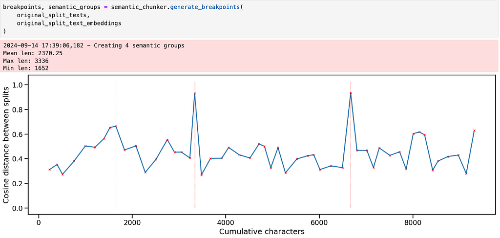
The pattern makes sense given what we know about the text — there are three big subjects, each of which has a few different sections. Aside from the two large spikes though, it’s not clear where the other breakpoints should be.

This is where the subjectivity and iteration comes in — depending on our application, we may want larger or smaller chunks and it’s important to use the graph to help guide our eye towards which chunks to actually read.

There are a few ways we could break the text into more granular chunks. The first is just to decrease the percentile threshold to make a breakpoint.

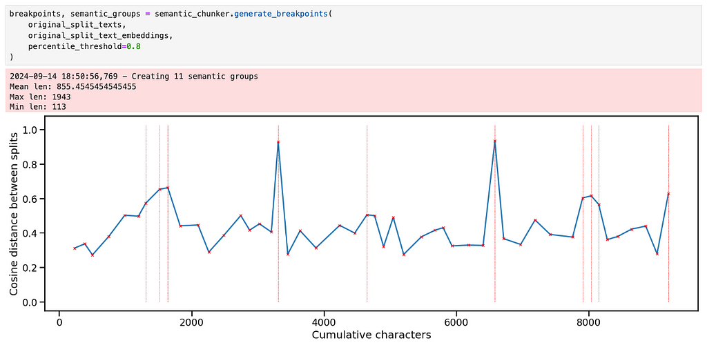
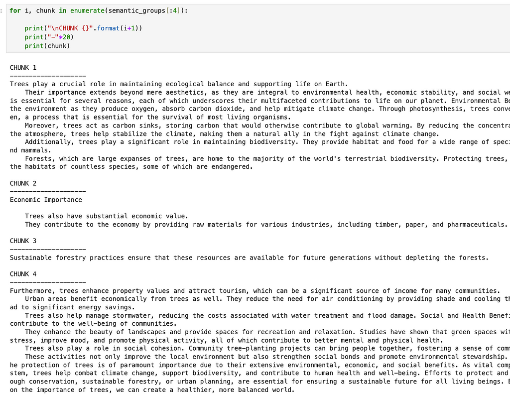
This creates 4 really small chunks and 8 larger ones. If we look at the first 4 chunks, for example, the splits seem semantically reasonable although I would argue that the 4th chunk is a bit too long, given that it contains most of the “economic importance”, “social importance” and “conclusions” sections of the first essay.

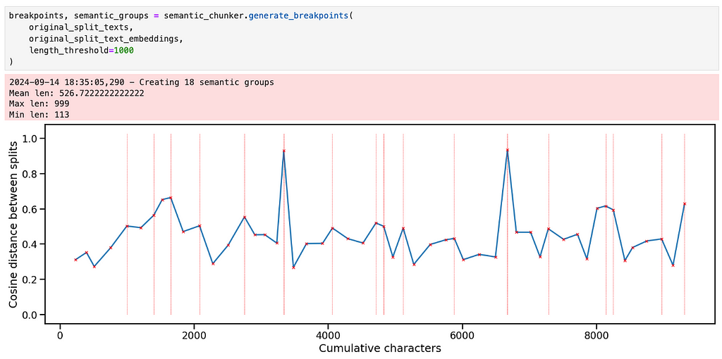
Instead of just changing the percentile threshold, an alternative idea is to apply the same threshold recursively. We start by creating breakpoints on the whole text. Then for each newly created chunk, if the chunk is above some length threshold, we create breakpoints just within that chunk. This happens until all the chunks are below the length threshold. Although somewhat subjective, I think this more closely mirrors what a human would do in that they would first identify very different groups of text and then iteratively reduce the size of each one.

It can be implemented with a stack, as shown below.

def get_breakpoints(
    embeddings: List[np.ndarray],
    start: int = 0,
    end: int = None,
    threshold: float = 0.95,
) -> np.ndarray:
    """
    Identifies breakpoints in embeddings based on cosine distance threshold.

    Args:
        embeddings (List[np.ndarray]): A list of embeddings.
        start (int, optional): The starting index for processing. Defaults to 0.
        end (int, optional): The ending index for processing. Defaults to None.
        threshold (float, optional): The percentile threshold for determining significant distance changes. Defaults to 0.95.

    Returns:
        np.ndarray: An array of indices where breakpoints occur.
    """
    if end is not None:
        embeddings_windowed = embeddings[start:end]
    else:
        embeddings_windowed = embeddings[start:]

    len_embeddings = len(embeddings_windowed)
    cdists = np.empty(len_embeddings - 1)
    
    # get the cosine distances between each chunk and the next one
    for i in range(1, len_embeddings):
        cdists[i - 1] = cosine(embeddings_windowed[i], embeddings_windowed[i - 1])
    
    # get the breakpoints
    difference_threshold = np.percentile(cdists, 100 * threshold, axis=0)
    difference_exceeding = np.argwhere(cdists >= difference_threshold).ravel()

    return difference_exceeding

def build_chunks_stack(
    self, length_threshold: int = 20000, cosine_distance_percentile_threshold: float = 0.95
) -> np.ndarray:
    """
    Builds a stack of text chunks based on length and cosine distance thresholds.

    Args:
        length_threshold (int, optional): Minimum length for a text chunk to be considered valid. Defaults to 20000.
        cosine_distance_percentile_threshold (float, optional): Cosine distance percentile threshold for determining breakpoints. Defaults to 0.95.

    Returns:
        np.ndarray: An array of indices representing the breakpoints of the chunks.
    """
    
    # self.split texts are the original split texts 
    # self.split text embeddings are their embeddings 
    S = [(0, len(self.split_texts))]
    all_breakpoints = set()
    while S:
        # get the start and end of this chunk
        id_start, id_end = S.pop()

        # get the breakpoints for this chunk
        updated_breakpoints = self.get_breakpoints(
            self.split_text_embeddings,
            start=id_start,
            end=id_end,
            threshold=cosine_distance_percentile_threshold,
        )
        updated_breakpoints += id_start

        # add the updated breakpoints to the set
        updated_breakpoints = np.concatenate(
            (np.array([id_start - 1]), updated_breakpoints, np.array([id_end]))
        )
        
        # for each updated breakpoint, add its bounds to the set and
        # to the stack if it is long enough
        for index in updated_breakpoints:
            text_group = self.split_texts[id_start : index + 1]
            if (len(text_group) > 2) and (
                self.get_text_length(text_group) >= length_threshold
            ):
                S.append((id_start, index))
            id_start = index + 1
        all_breakpoints.update(updated_breakpoints)
    
    # get all the breakpoints except the start and end (which will correspond to the start
    # and end of the text splits)
    return np.array(sorted(all_breakpoints))[1:-1]

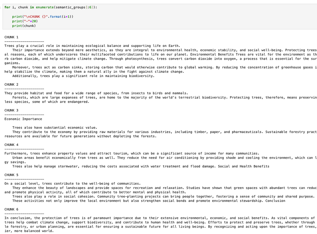
Our choice of length_threshold is also subjective and can be informed by the plot. In this case, a threshold of 1000 appears to work well. It divides the essays quite nicely into short and meaningfully different chunks.

Looking at the chunks corresponding to the first essay, we see that they are closely aligned with the different sections that GPT4-o created when it wrote the essay. Obviously in the case of this particular essay we could have just split on “nn” and been done here, but we want a more general approach.

2. Clustering the semantic splits

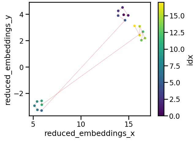
Now that we have made some candidate semantic chunks, it might be useful to see how similar they are to one another. This will help us get a sense for what information they contain. We will proceed by embedding the semantic chunks, and then use UMAP to reduce the dimensionality of the resulting embeddings to 2D so that we can plot them.

UMAP stands for Uniform Manifold Approximation and Projection, and is a powerful, general dimensionality reduction technique that can capture non-linear relationships. A full explanation of how it works can be found here. The purpose of using it here is to capture something of the relationships that exist between the embedded chunks in 1536-D space in a 2-D plot

from umap import UMAP

dimension_reducer = UMAP(
            n_neighbors=5, 
            n_components=2, 
            min_dist=0.0, 
            metric="cosine", 
            random_state=0
)
reduced_embeddings = dimension_reducer.fit_transform(semantic_embeddings)

splits_df = pd.DataFrame(
            {
                "reduced_embeddings_x": reduced_embeddings[:, 0],
                "reduced_embeddings_y": reduced_embeddings[:, 1],
                "idx": np.arange(len(reduced_embeddings[:, 0])),
            }
)

splits_df["chunk_end"] = np.cumsum([len(x) for x in semantic_text_groups])

ax = splits_df.plot.scatter(
            x="reduced_embeddings_x", 
            y="reduced_embeddings_y", 
            c="idx", 
            cmap="viridis"
)

ax.plot(
            reduced_embeddings[:, 0],
            reduced_embeddings[:, 1],
            "r-",
            linewidth=0.5,
            alpha=0.5,
)

UMAP is quite sensitive to the n_neighbors parameter. Generally the smaller the value of n_neighbors, the more the algorithm focuses on the use of local structure to learn how to project the data into lower dimensions. Setting this value too small can lead to projections that don’t do a great job of capturing the large scale structure of the data, and it should generally increase as the number of datapoints grows.

A projection of our data is shown below and its quite informative: Clearly we have three clusters of similar meaning, with the 1st and 3rd being more similar to each other than either is to the 2nd. The idx color bar in the plot above shows the chunk number, while the red line gives us an indication of the sequence of the chunks.

What about automatic clustering? This would be helpful if we wanted to group the chunks into larger segments or topics, which could serve as useful metadata to filter on in a RAG application with hybrid search, for example. We also might be able to group chunks that are far apart in the text (and therefore would not have been grouped by the standard semantic chunking in section 1) but have similar meanings.

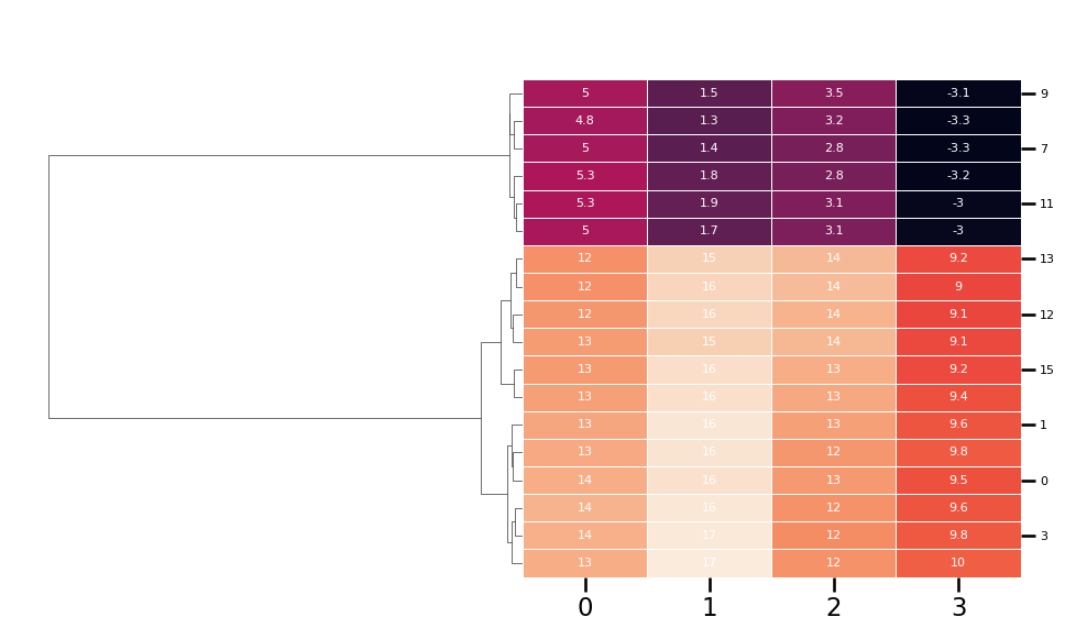
There are many clustering approaches that could be used here. HDBSCAN is a possibility, and is the default method recommended by the BERTopic package. However, in this case hierarchical clustering seems more useful since it can give us a sense of the relative importance of whatever groups emerge. To run hierarchical clustering, we first use UMAP to reduce the dimensionality of the dataset to a smaller number of components. So long as UMAP is working well here, the exact number of components shouldn’t significantly affect the clusters that get generated. Then we use the hierarchy module from scipy to perform the clustering and plot the result using seaborn

from scipy.cluster import hierarchy
from scipy.spatial.distance import pdist
from umap import UMAP
import seaborn as sns

# set up the UMAP
dimension_reducer_clustering = UMAP(
            n_neighbors=umap_neighbors,
            n_components=n_components_reduced,
            min_dist=0.0,
            metric="cosine",
            random_state=0
)
reduced_embeddings_clustering = dimension_reducer_clustering.fit_transform(
    semantic_group_embeddings
)

# create the hierarchy
row_linkage = hierarchy.linkage(
    pdist(reduced_embeddings_clustering),
    method="average",
    optimal_ordering=True,
)

# plot the heatmap and dendogram
g = sns.clustermap(
    pd.DataFrame(reduced_embeddings_clustering),
    row_linkage=row_linkage,
    row_cluster=True,
    col_cluster=False,
    annot=True,
    linewidth=0.5,
    annot_kws={"size": 8, "color": "white"},
    cbar_pos=None,
    dendrogram_ratio=0.5
)

g.ax_heatmap.set_yticklabels(
  g.ax_heatmap.get_yticklabels(), rotation=0, size=8
)

The result is also quite informative. Here n_components_reduced was 4, so we reduced the dimensionality of the embeddings to 4D, therefore making a matrix with 4 features where each row represents one of the semantic chunks. Hierarchical clustering has identified the two major groups (i.e. trees and Namibia), two large subgroup within trees (i.e. medical uses vs. other) and an number of other groups that might be worth exploring.

Note that BERTopic uses a similar technique for topic visualization, which could be seen as an extension of what’s being presented here.

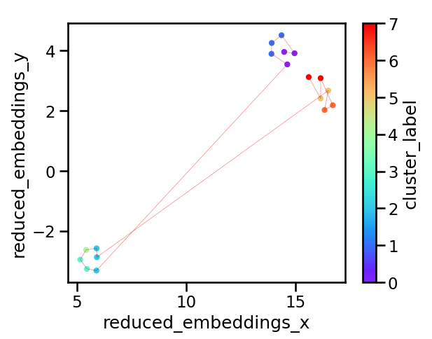
How is this useful in our exploration of semantic chunking? Depending on the results, we may choose to group some of the chunks together. This is again quite subjective and it might be important to try out a few different types of grouping. Let’s say we looked at the dendrogram and decided we wanted 8 distinct groups. We could then cut the hierarchy accordingly, return the cluster labels associated with each group and plot them.

cluster_labels = hierarchy.cut_tree(linkage, n_clusters=n_clusters).ravel()
dimension_reducer = UMAP(
  n_neighbors=umap_neighbors, 
  n_components=2, 
  min_dist=0.0, 
  metric="cosine", 
  random_state=0
)
reduced_embeddings = dimension_reducer.fit_transform(semantic_embeddings)

splits_df = pd.DataFrame(
            {
                "reduced_embeddings_x": reduced_embeddings[:, 0],
                "reduced_embeddings_y": reduced_embeddings[:, 1],
                "cluster_label": cluster_labels,
            }
        )

splits_df["chunk_end"] = np.cumsum(
            [len(x) for x in semantic_text_groups]
        ).reshape(-1, 1)

ax = splits_df.plot.scatter(
            x="reduced_embeddings_x",
            y="reduced_embeddings_y",
            c="cluster_label",
            cmap="rainbow",
        )

ax.plot(
  reduced_embeddings[:, 0],
  reduced_embeddings[:, 1],
  "r-",  
  linewidth=0.5,
  alpha=0.5,
)

The resulting plot is shown below. We have 8 clusters, and their distribution in the 2D space looks reasonable. This again demonstrates the importance of visualization: Depending on the text, application and stakeholders, the right number and distribution of groups will likely be different and the only way to check what the algorithm is doing is by plotting graphs like this.

3. Labeling the clusters

Assume after a few iterations of the steps above, we’ve settled on semantic splits and clusters that we’re happy with. It then makes sense to ask what these clusters actually represent? Obviously we could read the text and find out, but for a large corpus this is impractical. Instead, let’s use an LLM to help. Specifically, we will feed the text associated with each cluster to GPT-4o-mini and ask it to generate a summary. This is a relatively simple task with LangChain, and the core aspects of the code are shown below

import langchain
from langchain.prompts import PromptTemplate
from langchain_core.output_parsers.string import StrOutputParser
from langchain.callbacks import get_openai_callback
from dataclasses import dataclass


@dataclass
class ChunkSummaryPrompt:
    system_prompt: str = """
        You are an expert at summarization and information extraction from text. You will be given a chunk of text from a document and your
        task is to summarize what's happening in this chunk using fewer than 10 words. 

        Read through the entire chunk first and think carefully about the main points. Then produce your summary.

        Chunk to summarize: {current_chunk}
    """

    prompt: langchain.prompts.PromptTemplate = PromptTemplate(
        input_variables=["current_chunk"],
        template=system_prompt,
    )

class ChunkSummarizer(object):
    def __init__(self, llm):
        self.prompt = ChunkSummaryPrompt()
        self.llm = llm
        self.chain = self._set_up_chain()

    def _set_up_chain(self):
        return self.prompt.prompt | self.llm | StrOutputParser()

    def run_and_count_tokens(self, input_dict):
        with get_openai_callback() as cb:
            result = self.chain.invoke(input_dict)

        return result, cb

llm_model = "gpt-4o-mini"
llm = ChatOpenAI(model=llm_model, temperature=0, api_key=api_key)
summarizer = ChunkSummarizer(llm)

Running this on our 8 clusters and plotting the result with datamapplot gives the following

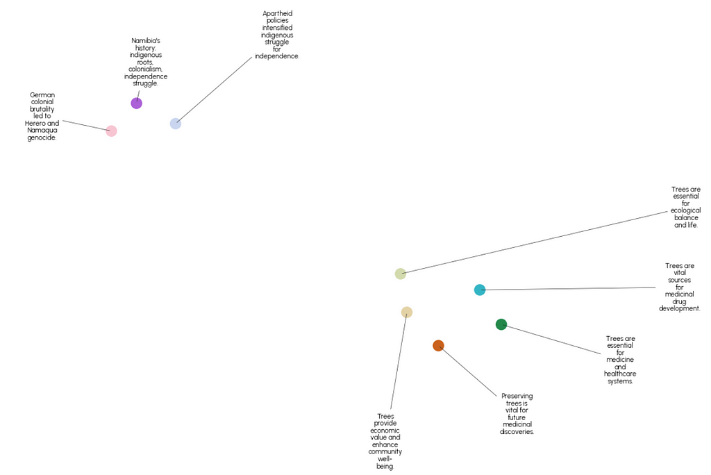
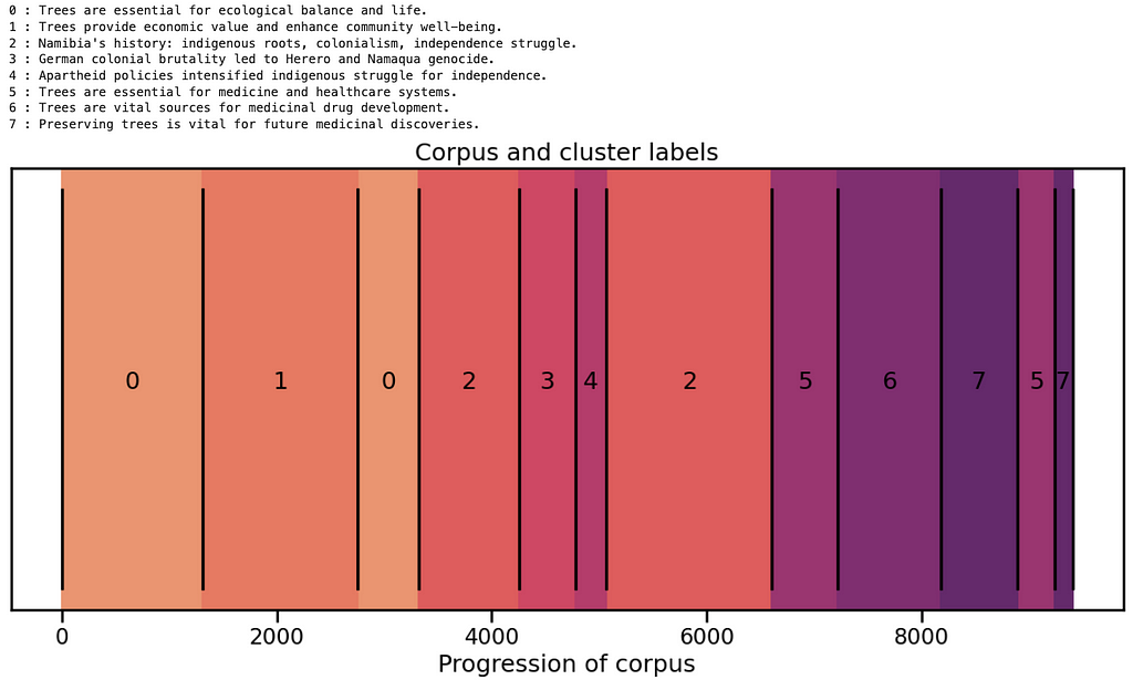
An alternative way of visualizing these groups is similar to the graphs shown in section 2, where we plot cumulative character number on the x axis and show the boundaries between the groups. Recall that we had 18 semantic chunks and have now grouped them further into 8 clusters. Plotting them like this shows how the semantic content of the text changes from beginning to end, highlights the fact that similar content is not always adjacent and gives a visual indication of the relative size of the chunks.

The code used to produce these figures can be found here.

4. Testing on a larger corpus

So far we’ve tested this workflow on a relatively small amount of text for demo purposes. Ideally it would also be useful on a larger corpus without significant modification. To test this, let’s try it out on a book downloaded from Project Gutenberg, and I’ve chosen the Wizard of Oz here. This is a much more difficult task because novels are typically not arranged in clear semantically distinct sections like factual essays. Although they are commonly arranged in chapters, the story line may “arch” in a continuous fashion, or skip around between different subjects. It would be very interesting to see if semantic chunk analysis could be used to learn something about the style of different authors from their work.

Step 1: Embed and generate breakpoints

from text_chunking.SemanticClusterVisualizer import SemanticClusterVisualizer
from text_chunking.utils.secrets import load_secrets
from text_chunking.datasets.test_text_dataset import TestText, TestTextNovel
from langchain_text_splitters import RecursiveCharacterTextSplitter

secrets = load_secrets()
semantic_chunker = SemanticClusterVisualizer(api_key=secrets["OPENAI_API_KEY"])

splitter = RecursiveCharacterTextSplitter(
        chunk_size=250,
        chunk_overlap=0,
        separators=["nn", "n", "."],
        is_separator_regex=False
)

original_split_texts = semantic_chunker.split_documents(
    splitter, 
    TestTextNovel.testing_text, 
    min_chunk_len=100, 
    verbose=True
)
original_split_text_embeddings = semantic_chunker.embed_original_document_splits(original_split_texts)

breakpoints, semantic_groups = semantic_chunker.generate_breakpoints(
    original_split_texts,
    original_split_text_embeddings,
    length_threshold=10000 #may need some iteration to find a good value for this parameter
)

This generates 77 semantic chunks of varying size. Doing some spot checks here led me to feel confident that it was working relatively well and many of the chunks end up being divided on or close to chapter boundaries, which makes a lot of sense.

Step 2 : Cluster and generate labels

On looking at the hierarchical clustering dendrogram, I decided to experiment with reduction to 35 clusters. The result reveals an outlier in the top left of the plot below (cluster id 34), which turns out to be a group of chunks at the very end of the text that contain a lengthy description of the terms under which the book is distributed.

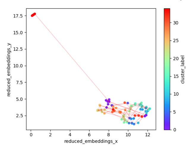
The descriptions given to each of the clusters are shown below and, with the exception of the first one, they provide a nice overview of the main events of the novel. A quick check on the actual texts associated with each one confirms that they are reasonably accurate summaries, although again, a determination of where the boundaries of the clusters should be is very subjective.

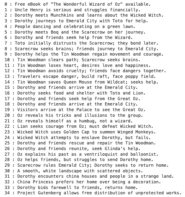
GPT-4o-mini labeled the outlier cluster “Project Gutenberg allows free distribution of unprotected works”. The text associated with this label is not particularly interesting to us, so let’s remove it and re-plot the result. This will make the structure in the novel easier to see.

What if we are interested in larger clusters? If we were to focus on high level structure, the dendrogram suggests approximately six clusters of semantic chunks, which are plotted below.

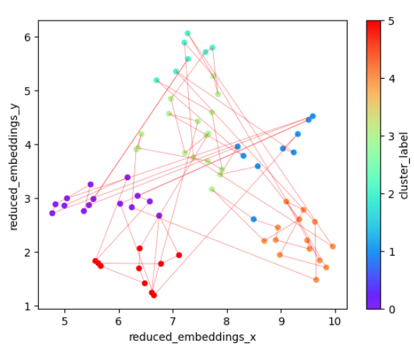
There’s a lot of jumping back and forth between points that are somewhat distant in this semantic space, suggesting frequent sudden changes in subject. It’s also interesting to consider the connectivity between the various clusters: 4 and 5 have no links between them for example, while there’s a lot of back and forth between 0 and 1.

Can we summarize these larger clusters? It turns out that our prompt doesn’t seem well suited for chunks of this size, producing descriptions that seem either too specific to one part of the cluster (i.e. clusters 0 and 4) or too vague to be very helpful. Improved prompt engineering — possibly involving multiple summarization steps — would probably improve the results here.

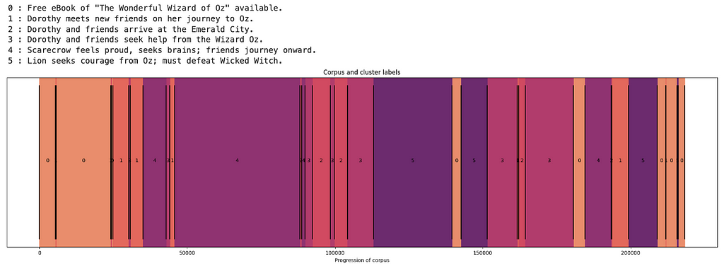
Despite the unhelpful names, this plot of the text segments colored by cluster is still informative as a guide to selective reading of the text. We see that the book starts and ends on the same cluster, which likely is about descriptions of Dorothy, Toto and their home — and aligns with the story arch of the Wizard of Oz as a journey and subsequent return. Cluster 1 is mainly about meeting new characters, which happens mainly near the beginning but also periodically throughout the book. Clusters 2 and 3 are concerned with Emerald City and the Wizard, while clusters 4 and 5 are broadly about journeying and fighting respectively.

5. Concluding thoughts

Thanks for making it to the end! Here we took a deep dive into the idea of semantic chunking, and how it can be complimented by dimensionality reduction, clustering and visualization. The major takeaway is the importance of systematically exploring the effects of different chunking techniques and a parameters on your text before deciding on the most suitable approach. My hope is that this article will spark new ideas about how we can use AI and visualization tools to advance semantic chunking and quickly extract insights from large bodies of text. Please feel free to explore the full codebase here https://github.com/rmartinshort/text_chunking.

A Visual Exploration of Semantic Text Chunking was originally published in Towards Data Science on Medium, where people are continuing the conversation by highlighting and responding to this story.