Does Semi-Supervised Learning Help to Train Better Models?

Evaluating how semi-supervised learning can leverage unlabeled data

One of the most common challenges Data Scientists faces is the lack of enough labelled data to train a reliable and accurate model. Labelled data is essential for supervised learning tasks, such as classification or regression. However, obtaining labelled data can be costly, time-consuming, or impractical in many domains. On the other hand, unlabeled data is usually easy to collect, but they do not provide any direct input to train a model.

How can we make use of unlabeled data to improve our supervised learning models? This is where semi-supervised learning comes into play. Semi-supervised learning is a branch of machine learning that combines labelled and unlabeled data to train a model that can perform better than using labelled data alone. The intuition behind semi-supervised learning is that unlabeled data can provide useful information about the underlying structure, distribution, and diversity of the data, which can help the model generalize better to new and unseen examples.

In this post, I present three semi-supervised learning methods that can be applied to different types of data and tasks. I will also evaluate their performance on a real-world dataset and compare them with the baseline of using only labelled data.

What is semi-supervised learning?

Semi-supervised learning is a type of machine learning that uses both labelled and unlabeled data to train a model. Labelled data are examples that have a known output or target variable, such as the class label in a classification task or the numerical value in a regression task. Unlabeled data are examples that do not have a known output or target variable. Semi-supervised learning can leverage the large amount of unlabeled data that is often available in real-world problems, while also making use of the smaller amount of labelled data that is usually more expensive or time-consuming to obtain.

The underlying idea to use unlabeled data to train a supervised learning method is to label this data via supervised or unsupervised learning methods. Although these labels are most likely not as accurate as actual labels, having a significant amount of this data can improve the performance of a supervised-learning method compared to training this method on labelled data only.

The scikit-learn package provides three semi-supervised learning methods:

• Self-training: a classifier is first trained on labelled data only to predict labels of unlabeled data. In the next iteration, another classifier is training on the labelled data and on prediction from the unlabeled data which had high confidence. This procedure is repeated until no new labels with high confidence are predicted or a maximum number of iterations is reached.
• Label-propagation: a graph is created where nodes represent data points and edges represent similarities between them. Labels are iteratively propagated through the graph, allowing the algorithm to assign labels to unlabeled data points based on their connections to labelled data.
• Label-spreading: uses the same concept as label-propagation. The difference is that label spreading uses a soft assignment, where the labels are updated iteratively based on the similarity between data points. This method may also “overwrite” labels of the labelled dataset.

To evaluate these methods I used a diabetes prediction dataset which contains features of patient data like age and BMI together with a label describing if the patient has diabetes. This dataset contains 100,000 records which I randomly divided into 80,000 training, 10,000 validation and 10,000 test data. To analyze how effective the learning methods are with respect to the amount of labelled data, I split the training data into a labelled and an unlabeled set, where the label size describes how many samples are labelled.

I used the validation data to assess different parameter settings and used the test data to evaluate the performance of each method after parameter tuning.

I used XG Boost for prediction and F1 score to evaluate the prediction performance.

Baseline

The baseline was used to compare the self-learning algorithms against the case of not using any unlabeled data. Therefore, I trained XGB on labelled data sets of different size and calculate the F1 score on the validation data set:

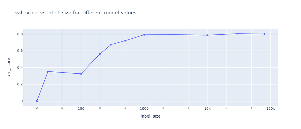
The results showed that the F1 score is quite low for training sets of less than 100 samples, then steadily improves to a score of 79% until a sample size of 1,000 is reached. Higher sample sizes hardly improved the F1 score.

Self-learning

Self-training is using multiple iteration to predict labels of unlabeled data which will then be used in the next iteration to train another model. Two methods can be used to select predictions to be used as labelled data in the next iteration:

1. Threshold (default): all predictions with a confidence above a threshold are selected
2. K best: the predictions of the k highest confidence are selected

I evaluated the default parameters (ST Default) and tuned the threshold (ST Thres Tuned) and the k best (ST KB Tuned) parameter based on the validation dataset. The prediction results of these model were evaluated on the test dataset:

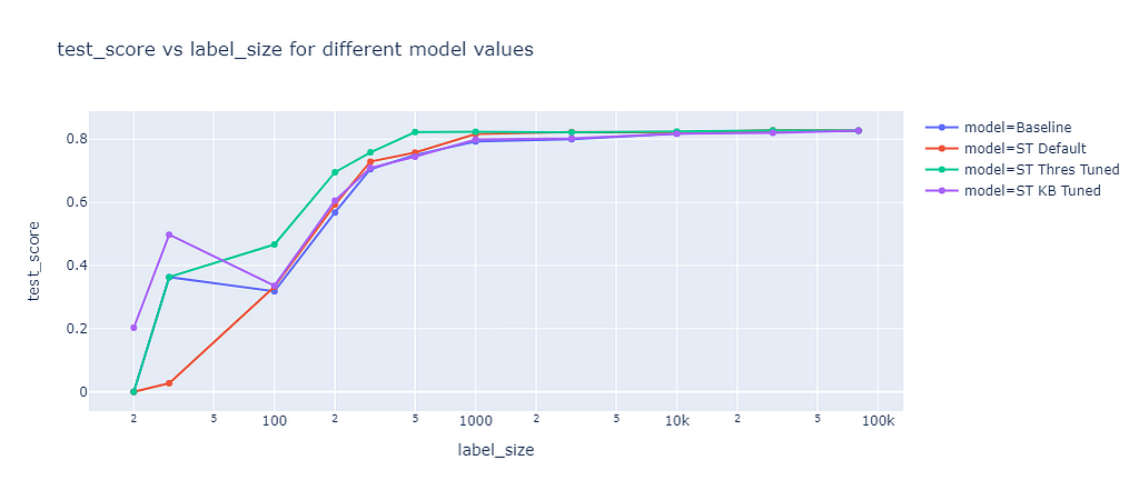
For small sample sizes (<100) the default parameters (red line) performed worse than the baseline (blue line). For higher sample sizes slightly better F1 scores than the baseline were achieved. Tuning the threshold (green line) brought a significant improvement, for example at a label size of 200 the baseline F1 score was 57% while the algorithm with tuned thresholds achieved 70%. With one exception at a label size of 30, tuning the K best value (purple line) resulted in almost the same performance as the baseline.

Label Propagation

Label propagation has two built-in kernel methods: RBF and KNN. The RBF kernel produces a fully connected graph using a dense matrix, which is memory intensive and time consuming for large datasets. To consider memory constraints, I only used a maximum training size of 3,000 for the RBF kernel. The KNN kernel uses a more memory friendly sparse matrix, which allowed me to fit on the whole training data of up to 80,000 samples. The results of these two kernel methods are compared in the following graph:

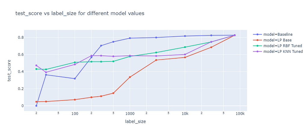
The graph shows the F1 score on the test dataset of different label propagation methods as a function of the label size. The blue line represents the baseline, which is the same as for self-training. The red line represents the label propagation with default parameters, which clearly underperforms the baseline for all label sizes. The green line represents the label propagation with RBF kernel and tuned parameter gamma. Gamma defines how far the influence of a single training example reaches. The tuned RBF kernel performed better than the baseline for small label sizes (<=100) but worse for larger label sizes. The purple line represents the label propagation with KNN kernel and tuned parameter k, which determines the number of nearest neighbors to use. The KNN kernel had a similar performance as the RBF kernel.

Label Spreading

Label spreading is a similar approach to label propagation, but with an additional parameter alpha that controls how much an instance should adopt the information of its neighbors. Alpha can range from 0 to 1, where 0 means that the instance keeps its original label and 1 means that it completely adopts the labels of its neighbors. I also tuned the RBF and KNN kernel methods for label spreading. The results of label spreading are shown in the next graph:

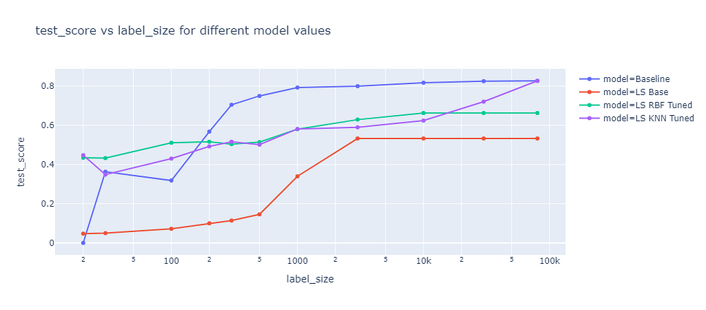
The results of label spreading were very similar to those of label propagation, with one notable exception. The RBF kernel method for label spreading has a lower test score than the baseline for all label sizes, not only for small ones. This suggests that the “overwriting” of labels by the neighbors’ labels has a rather negative effect for this dataset, which might have only few outliers or noisy labels. On the other hand, the KNN kernel method is not affected by the alpha parameter. It seems that this parameter is only relevant for the RBF kernel method.

Comparison of all methods

Next, I compared all methods with their best parameters against each other.

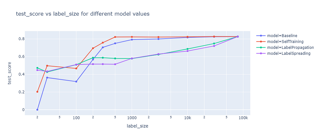
The graph shows the test score of different semi-supervised learning methods as a function of the label size. Self-training outperforms the baseline, as it leverages the unlabeled data well. Label propagation and label spreading only beat the baseline for small label sizes and perform worse for larger label sizes.

Conclusion

The results may significantly vary for different datasets, classifier methods, and metrics. The performance of semi-supervised learning depends on many factors, such as the quality and quantity of the unlabeled data, the choice of the base learner, and the evaluation criterion. Therefore, one should not generalize these findings to other settings without proper testing and validation.

If you are interested in exploring more about semi-supervised learning, you are welcome to check out my git repo and experiment on your own. You can find the code and data for this project here.

One thing that I learned from this project is that parameter tuning was important to significantly improve the performance of these methods. With optimized parameters, self-training performed better than the baseline for any label size and reached better F1 scores of up to 13%! Label propagation and label spreading only turned out to improve the performance for very small sample size, but the user must be very careful not to get worse results compared to not using any semi-supervised learning method.

Does Semi-Supervised Learning Help to Train Better Models? was originally published in Towards Data Science on Medium, where people are continuing the conversation by highlighting and responding to this story.