VAE for Time Series

Generate realistic sequential data with this easy-to-train model

Variational autoencoders (VAEs) are a form of generative AI that came into the spotlight for their ability to create realistic images, but they can also create compelling time series. The standard VAE can be adapted to capture periodic and sequential patterns of time series data, and then be used to generate plausible simulations. The model I built simulates temperature data using 1-D convolution layers, a strategic choice of strides, a flexible time dimension, and a seasonally dependent prior.

Objective

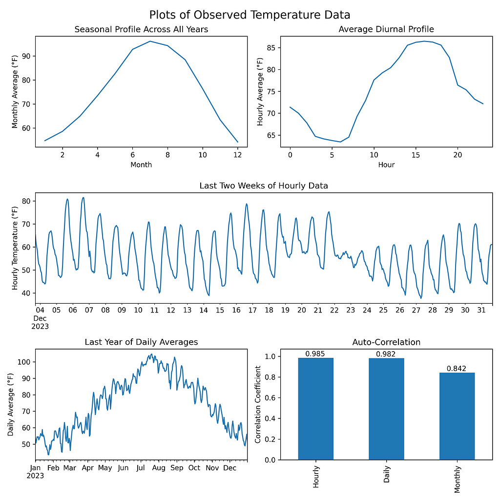
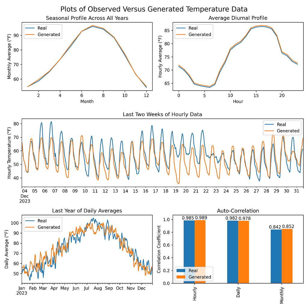
I trained a model on 50 years of hourly ERA5 temperature data from Phoenix, Arizona [1]. To have useful generated data, it must capture a few characteristics of the original data:

1. seasonal profile — summers should be warmer than winters
2. diurnal profile — days should be warmer than nights
3. autocorrelation—the data should be smooth, and consecutive days should have similar temperatures

Impact of Climate Change

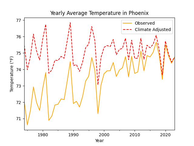
The model performs best if the training data is stationary, without a long-term trend. However, due to climate change, the temperature trends upward by about 0.7 °F per decade — a value derived from the observed data which is consistent with published maps showing recent warming trends by region [2]. To account for the increasing temperature, I applied a -0.7 °F per decade linear transformation to the raw observations to erase the upward trend. This adjusted dataset represents what historical temperatures may have looked like if we assume 2024’s climate conditions. Interpretations of the the generated data should keep this in mind.

What is a VAE?

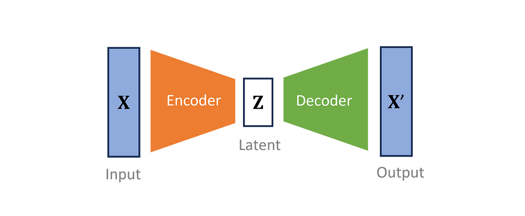
Variational autoencoders reduce the dimensions of the input data into a smaller subspace. VAEs define an encoder to transform observed inputs into a compressed form called the latent variable. Then, a distinct, mirroring decoder attempts to recreate the original data. The encoder and decoder are co-optimized to make an encoding that loses as little information as possible.

The full loss function used in training includes:

• a reconstruction loss: measuring how closely the round-trip, transformed data matches the original inputs
• a regularization term: measuring how closely the encoded distribution for the latent variable matches the prior distribution.

These two loss terms are derived using variational inference by trying to maximize the evidence lower bound (ELBO) of the observed data. Check out this video for the mathematical derivation [3].

Intuitively, VAEs perform feature extraction on the training data in such a way that the most important features, represented by the latent variable, follow the defined prior distribution. New data is generated by sampling the latent distribution and then decoding it to the form of the original inputs.

Check out Joseph Rocca’s article, Understanding Variational Autoencoders, for a more thorough explanation of how VAEs work [4].

1-D convolutional layers

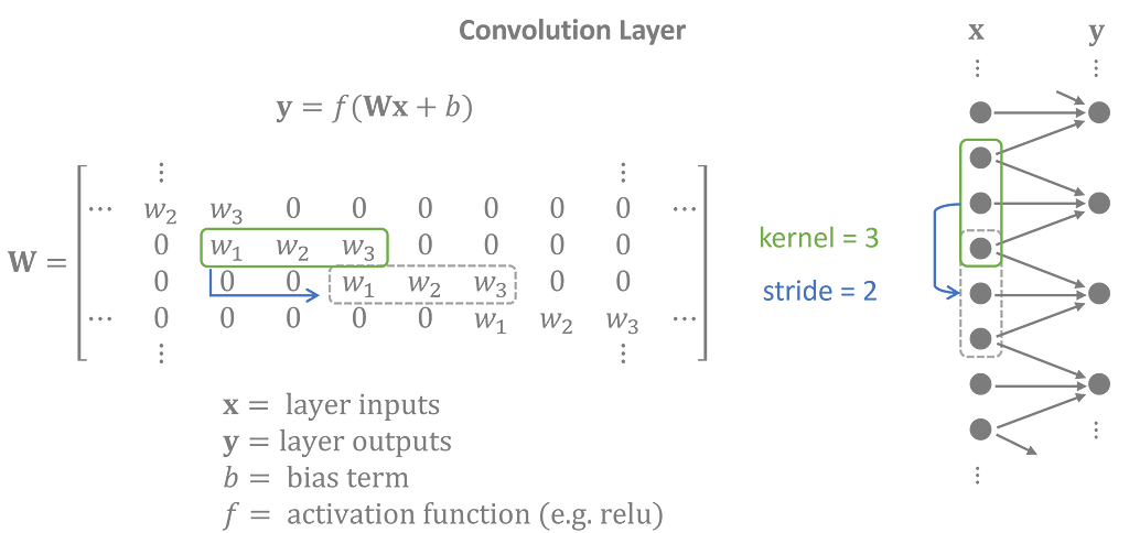
For modeling Phoenix temperature data, I made my encoder a neural network with one-dimensional convolutional layers. Each convolution layer applies a kernel — a matrix of weights — to shifted intervals of the inputs. Since the same kernel is used across the entire input, convolutional layers are considered shift invariant and are well suited for time series which have repeating patterns of sequences.

The decoder performs the opposite task of the encoder with transposed 1-D convolutional layers, also called deconvolution layers. Latent features are projected into overlapping sequences to create an output time series that closely matches the inputs.

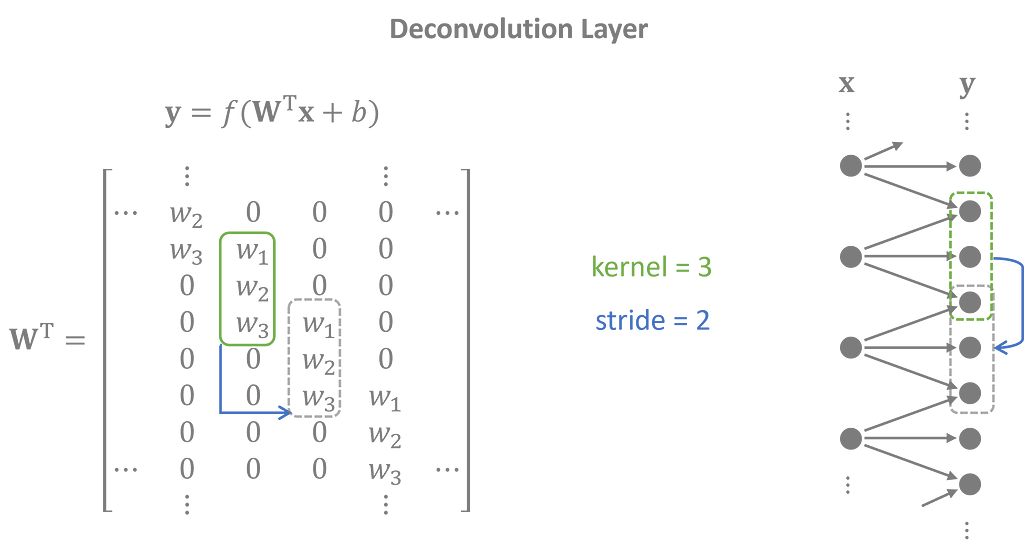
The full model stacks several convolution and deconvolution layers together. Each intermediate, hidden layer extends the range of the latent variables allowing the model to capture long-range effects in the data.

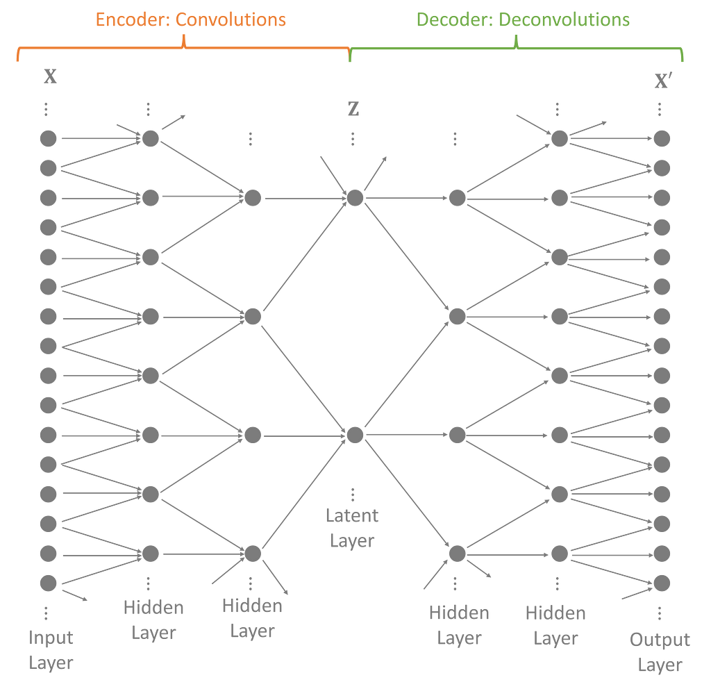
Strategic Strides

The stride — the jump between shifts — determines the size of the next layer. Convolution layers use strides to shrink the inputs down, and deconvolution layers use strides to expand the latent variables back to the input size. However, they also serve a secondary purpose — to capture periodic trends in the time series.

You can strategically select the strides of the convolution layers to replicate the periodic patterns in the data.

Convolutions apply the kernel cyclically, repeating the same weights with a period equal to its stride. This gives the training process the freedom to customize the weights based on the input’s position in the cycle.

Stacking multiple layers together results in a larger effective period made of nested sub-convolutions.

Consider a convolutional network that distills hourly time series data into a features space with four variables per day representing morning, afternoon, evening, and night. A layer with a stride of 4 will have weights uniquely assigned to each time of day that captures the diurnal profile in the hidden layer. During training, the encoder and decoder learn weights that replicate the daily cycles found in the data.

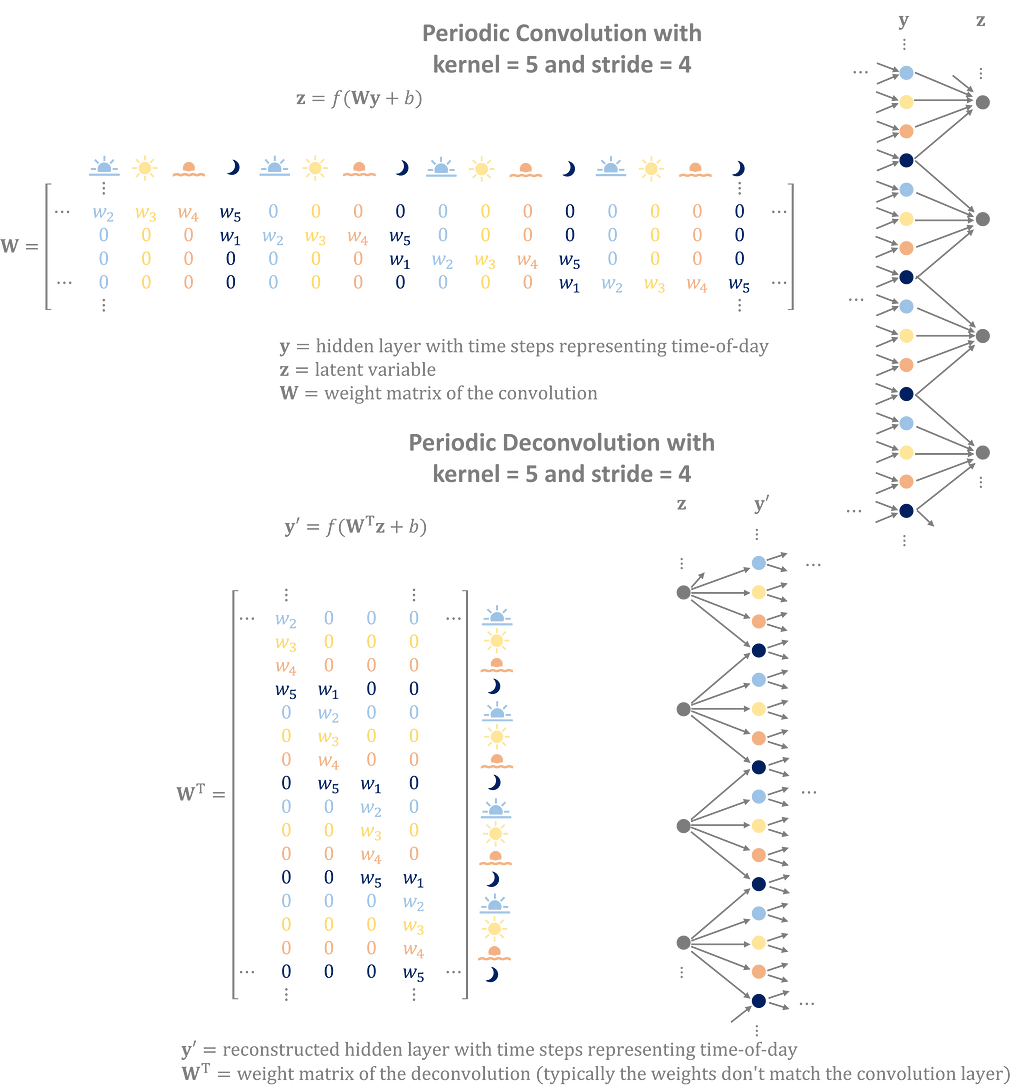
Convolutions exploit the cyclical nature of the inputs to build better latent features. Deconvolutions convert latent features into overlapping, repeating sequences to generate data with periodic patterns.

Flexible Time Dimension

Image-generating VAEs usually have thousands of images pre-processed to have a fixed width and height. The generated images will match the width and height of the training data.

For the Phoenix dataset, I only have one 50 year time series. To improve the training, I broke the data up into sequences, ultimately settling on assigning a latent variable to each 96 hour period. However, I may want to generate time series that are longer than 4 days, and, ideally, the output is smooth rather than having discrete 96 hour chunks in the simulations.

Fortunately, Tensorflow allows you to specify unconstrained dimensions in your neural network. In the same way that neural networks can handle any batch size, you can build your model to handle an arbitrary number of time steps. As a result, my latent variable also includes a time dimension which can vary. In my model, there is one time step in the latent space for every 96 hours in the inputs.

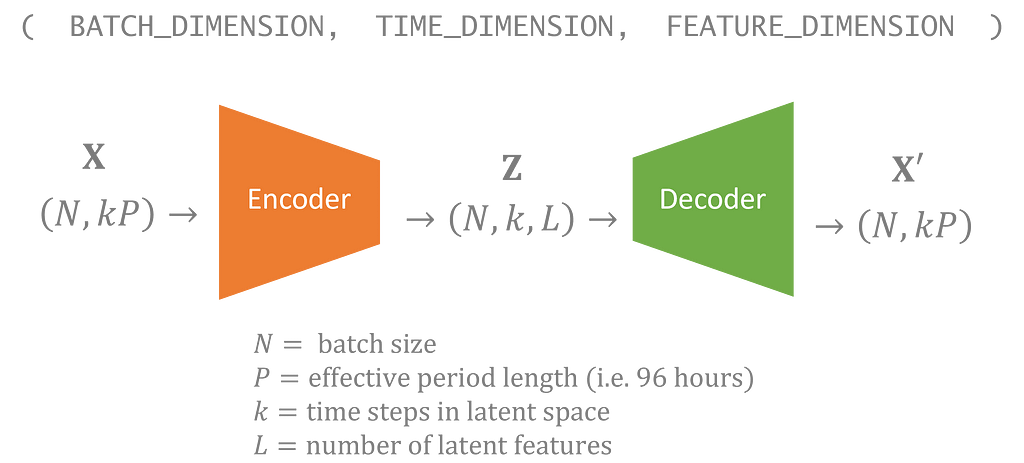
Generating new data is as simple as sampling latent variables from the prior where you select the number of steps you want to include in the time dimension.

VAEs with an unconstrained time dimension can generate data to any length.

The simulated output will have 4 days for each time step you sampled, and the results will appear smooth since convolution layers allow input layers to spill into neighboring time periods.

Seasonally dependent prior

In most VAEs, each component of the latent variable is assumed to follow a standard normal distribution. This distribution, sometimes called the prior, is sampled, then decoded, to generate new data. In this case, I chose a slightly more complex prior that depends on the time of year.

Latent variables sampled from a seasonal prior will generate data with characteristics that vary by the time of year.

Under this prior, generated January data will look very different than July data, and generated data from the same month will share many of the same features.

I represented the time of year as an angle, θ, where 0° is January 1st, 180° is the beginning of July, and 360° is back to January again. The prior is a normal distribution whose mean and log-variance is a third degree trigonometric polynomial of θ where the coefficients of the polynomial are parameters learned during training in conjunction with the encoder and decoder.

The prior distribution parameters are a periodic function of θ, and well-behaved periodic functions can be approximated to any level of accuracy given a trigonometric polynomial of sufficiently high degree. [5]

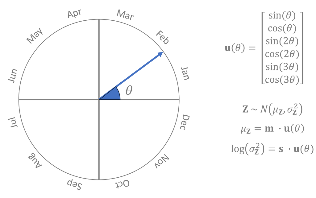
The seasonal data is only used in the prior and doesn’t influence the encoder or decoder. The full set of probabilistic dependencies is shown here graphically.

Implementation

I trained the model using Tensorflow in Python.

from tensorflow.keras import layers, models

Encoder

The input is defined with a flexible time dimension. In Keras, you specify an unconstrained dimension using None .

Using the ‘same’ padding will append zeros to the input layer such that the output size matches the input size divided by the stride.

inputs = layers.Input(shape=(None,)) # (N, 96*k)
x = layers.Reshape((-1, 1))(inputs)  # (N, 96*k, 1)

# Conv1D parameters: filters, kernel_size, strides, padding
x = layers.Conv1D(40, 5, 3, 'same', activation='relu')(x) # (N, 32*k, 40)
x = layers.Conv1D(40, 3, 2, 'same', activation='relu')(x) # (N, 16*k, 40)
x = layers.Conv1D(40, 3, 2, 'same', activation='relu')(x) # (N, 8*k, 40)
x = layers.Conv1D(40, 3, 2, 'same', activation='relu')(x) # (N, 4*k, 40)
x = layers.Conv1D(40, 3, 2, 'same', activation='relu')(x) # (N, 2*k, 40)
x = layers.Conv1D(20, 3, 2, 'same')(x) # (N, k, 20)

z_mean = x[: ,:, :10]   # (N, k, 10)
z_log_var = x[:, :, 10:] # (N, k, 10)
z = Sampling()([z_mean, z_log_var]) # custom layer sampling from gaussian

encoder = models.Model(inputs, [z_mean, z_log_var, z], name='encoder')

Sampling() is a custom layer that samples data from a normal distribution with the given mean and log variance.

Decoder

Deconvolution is performed with Conv1DTranspose .

# input shape: (batch_size, time_length/96, latent_features)
inputs = layers.Input(shape=(None, 10)) # (N, k, 10)

# Conv1DTranspose parameters: filters, kernel_size, strides, padding
x = layers.Conv1DTranspose(40, 3, 2, 'same', activation='relu')(inputs) # (N, 2*k, 40)
x = layers.Conv1DTranspose(40, 3, 2, 'same', activation='relu')(x) # (N, 4*k, 40)
x = layers.Conv1DTranspose(40, 3, 2, 'same', activation='relu')(x) # (N, 8*k, 40)
x = layers.Conv1DTranspose(40, 3, 2, 'same', activation='relu')(x) # (N, 16*k, 40)
x = layers.Conv1DTranspose(40, 3, 2, 'same', activation='relu')(x) # (N, 32*k, 40)
x = layers.Conv1DTranspose(1,  5, 3, 'same')(x) # (N, 96*k, 1)

outputs = layers.Reshape((-1,))(x) # (N, 96*k)

decoder = models.Model(inputs, outputs, name='decoder')

Prior

The prior expects inputs already in the form [sin(θ), cos(θ), sin(2θ), cos(2θ), sin(3θ), cos(3θ)].

The Dense layer has no bias term as a way of preventing the prior distribution from drifting too far from zero or having an overall variance that was too high or too small.

# seasonal inputs shape: (N, k, 6)
inputs = layers.Input(shape=(None, 2*3)) 

x = layers.Dense(20, use_bias=False)(inputs) # (N, k, 20)
z_mean = x[:, :, :10]  # (N, k, 10)
z_log_var = x[:, :, 10:] # (N, k, 10)
z = Sampling()([z_mean, z_log_var]) # (N, k, 10)

prior = models.Model(inputs, [z_mean, z_log_var, z], name='seasonal_prior')

Full Model

The loss function contains a reconstruction term and a latent regularization term.

Function log_lik_normal_sum is a custom function for calculating the normal log likelihood of the observed data given the reconstructed output. Calculating the log-likelihood requires noise distribution around the decoded output which is assumed to be normal with log variance given by self.noise_log_var, learned during training.

For the regularization term, kl_divergence_sum calculates the Kullback–Leibler divergence between two gaussians — in this case, the latent encoded and prior distributions.

class VAE(models.Model):
    def __init__(self, encoder, decoder, prior, **kwargs):
        super(VAE, self).__init__(**kwargs)
        self.encoder = encoder
        self.decoder = decoder
        self.prior = prior
        self.noise_log_var = self.add_weight(name='var', shape=(1,), initializer='zeros', trainable=True)

    @tf.function
    def vae_loss(self, data):
        values, seasonal = data
        z_mean, z_log_var, z = self.encoder(values)
        reconstructed = self.decoder(z)
        reconstruction_loss = -log_lik_normal_sum(values, reconstructed, self.noise_log_var)/INPUT_SIZE
        seasonal_z_mean, seasonal_z_log_var, _ = self.prior(seasonal)
        kl_loss_z = kl_divergence_sum(z_mean, z_log_var, seasonal_z_mean, seasonal_z_log_var)/INPUT_SIZE
        return reconstruction_loss, kl_loss_z

    def train_step(self, data):
        with tf.GradientTape() as tape:
            reconstruction_loss, kl_loss_z = self.vae_loss(data)
            total_loss = reconstruction_loss + kl_loss_z
        
        gradients = tape.gradient(total_loss, self.trainable_variables)
        self.optimizer.apply_gradients(zip(gradients, self.trainable_variables))
        
        return {'loss': total_loss}

For the full implementation, visit my Github repository.

Results

After training the model, the generated data matches the seasonal/diurnal profiles and autocorrelation of the original temperature data.

Conclusion

Building techniques for generative time series modeling is a crucial field with applications beyond just simulating data. The methods I shared could be adapted for applications in data imputation, anomaly detection, and forecasting.

By using 1-D convolutional layers, strategic strides, flexible time inputs, and seasonal priors, you can build a VAE that replicates complex patterns in your time series. Let’s collaborate to refine best practices for time series modeling.

Share in the comments any experience, questions, or insights you have with VAEs and/or generative AI for time series.

All images have been created by the author unless otherwise stated.

[1] Hersbach, H., Bell, B., Berrisford, P., Biavati, G., Horányi, A., Muñoz Sabater, J., Nicolas, J., Peubey, C., Radu, R., Rozum, I., Schepers, D., Simmons, A., Soci, C., Dee, D., Thépaut, J-N. (2023): ERA5 hourly data on single levels from 1940 to present. Copernicus Climate Change Service (C3S) Climate Data Store (CDS), DOI: 10.24381/cds.adbb2d47 (Accessed on 01-Aug-2024)

[2] Lindsey, R., & Dahlman, L. (2024, January 18). Climate change: Global temperature. Climate.gov. https://www.climate.gov/news-features/understanding-climate/climate-change-global-temperature

[3] Sachdeva, K. (2021, January 26). Evidence lower bound (ELBO) — Clearly explained! [Video]. YouTube. https://www.youtube.com/watch?v=IXsA5Rpp25w

[4] Rocca, J. (2019, September 23). Understanding variational autoencoders (VAEs). Towards Data Science. https://towardsdatascience.com/understanding-variational-autoencoders-vaes-f70510919f73

[5] Baidoo, F. A. (2015, August 28). Uniform convergence of Fourier series (REU Report). University of Chicago. https://math.uchicago.edu/~may/REU2015/REUPapers/Baidoo.pdf

VAE for Time Series was originally published in Towards Data Science on Medium, where people are continuing the conversation by highlighting and responding to this story.