Heckman Selection Bias Modeling in Causal Studies

How selection bias is related to the identification assumptions of OLS, and what steps should be taken to address it

Throughout my applied studies, I struggled to grasp the complexities of selection and sample bias problems. These issues manifest in various forms, can arise from different factors, and can affect both external and internal validity in causal models. Additionally, they are often the source of semantic confusion.

One of the foundational concepts to understand when addressing bias and inconsistencies in a linear causal model is the omitted variable problem. This occurs when a typically unobserved random variable is correlated with both the independent variable and the model error. Failing to account for this variable when estimating a linear model leads to biased estimators. Consequently, this problem hinders the isolation of variance in the dependent variable in response to changes in the independent variable, thus obscuring the true causal relationship between the two.

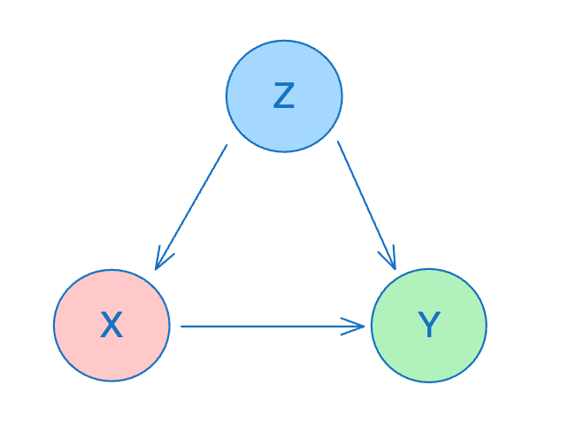
Are these concepts connected? Can selection bias be considered a form of the omitted variable problem? Let’s dive in and explore!

Background

I’d like to lay out the foundational elements needed to fully grasp how selection bias affects our linear model estimation process. We have a dependent random variable, Y, which we assume has a linear relationship (subject to some error terms) with another variable, X, known as the independent variable.

Identification Assumptions

Given a subsample Y’, X’ of the population variables Y, X –

1. The error terms (of the original model !!!) and X’ are not correlated.
2. The mean of the error terms is zero.
3. Y and X are really related in a linear way —

It’s important to note that in empirical research, we observe X and Y (or a subsample of them), but we don’t observe the error terms, making assumption (1) impossible to test or validate directly. At this point, we usually rely on a theoretical explanation to justify this assumption. A common justification is through randomized controlled trials (RCTs), where the subsample, X, is collected entirely at random, ensuring that it is uncorrelated with any other variable, particularly with the error terms.

Conditional Expectation

Given the assumptions mentioned earlier, we can precisely determine the form of the conditional expectation of Y given X —

The last transition follows from the identification assumptions. It’s important to note that this is a function of x, meaning it represents the average of all observed values of y given that x is equal to a specific value (Or the local average of y’s given a small range of values of x’s — more information can be found here)

OLS

Given a sample of X that meets the identification assumptions, it’s well-established that the ordinary least squares (OLS) method provides a closed-form solution for consistent and unbiased estimators of the linear model parameters, alpha and beta, and thus for the conditional expectation function of Y given X.

At its core, OLS is a technique for fitting a linear line (or linear hyperplane in the case of a multivariate sample) to a set of (y_i, x_i) pairs. What’s particularly interesting about OLS is that —

1. If Y and X have a linear relationship (accounting for classic error terms), we’ve seen that the conditional expectation of Y given X is perfectly linear. In this scenario, OLS effectively uncovers this function with strong statistical accuracy.
2. OLS achieves this even with any subsample of X that meets the identification assumptions previously discussed — with large enough sample.

Motivation

Let’s begin with a straightforward example using simulated data. We’ll simulate the linear model from above.

A significant advantage of working with simulated data is that it allows us to better understand relationships between variables that are not observable in real-world scenarios, such as the error terms in the model.

import matplotlib.pyplot as plt
import numpy as np
import pandas as pd
import statsmodels.api as sm

N = 5000
BETA = 0.7
INTERCEPT = -2
SIGMA = 5

df = pd.DataFrame({
    "x": np.random.uniform(0, 50, N),
    "e": np.random.normal(0, SIGMA, N)
})
df["y"] = INTERCEPT + BETA * df["x"] + df["e"]

and running OLS for the full sample –

r1 = sm.OLS(df["y"], sm.add_constant(df["x"])).fit()
plt.scatter(df["x"], df["y"], label="population")
plt.plot(df["x"], r1.fittedvalues, label="OLS Population", color="r")

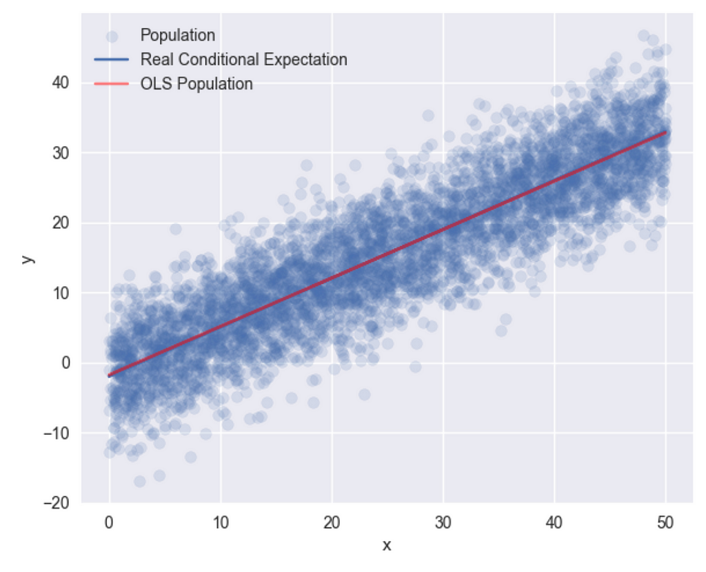
Now, let’s generate a random subsample of our population, X, and apply OLS to this subsample. I’ll randomly select 100 x’s from the 500 samples I previously generated, and then run OLS on this subset.

sample1 = df.sample(100)
r2 = sm.OLS(sample1["y"], sm.add_constant(sample1["x"])).fit()

plt.scatter(sample1["x"], sample1["y"], label="sample")
plt.plot(sample1["x"], r2.fittedvalues, label="OLS Random sample")

and plot –

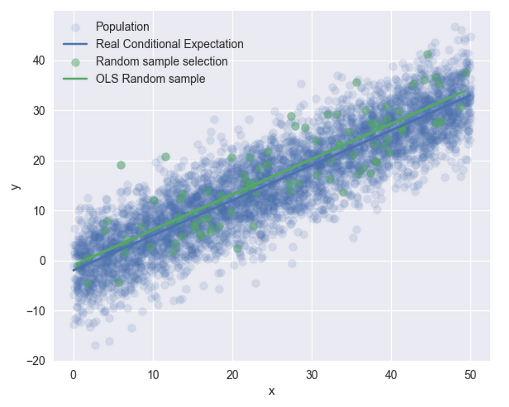
It appears we obtain consistent estimators for the random subsample, as both OLS results produce quite similar conditional expectation lines. Additionally, you can observe the correlation between X and the error terms —

print(f"corr {np.corrcoef(df['x'], df['e'])}")
print(f"E(e|x) {np.mean(df['e'])}")

# corr [[ 1.         -0.02164744]
#  [-0.02164744  1.        ]]
# E(e|x) 0.004016713100777963

This suggests that the identification assumptions are being met. In practice, however, we cannot directly calculate these since the errors are not observable. Now, let’s create a new subsample — I’ll select all (y, x) pairs where y ≤ 10:

sample2 = df[df["y"] <= 10]
r3 = sm.OLS(sample2["y"], sm.add_constant(sample2["x"])).fit()

plt.scatter(sample2["x"], sample2["y"], label="Selected sample")
plt.plot(sample["x"], r3.fittedvalues, label="OLS Selected Sample")

and we get –

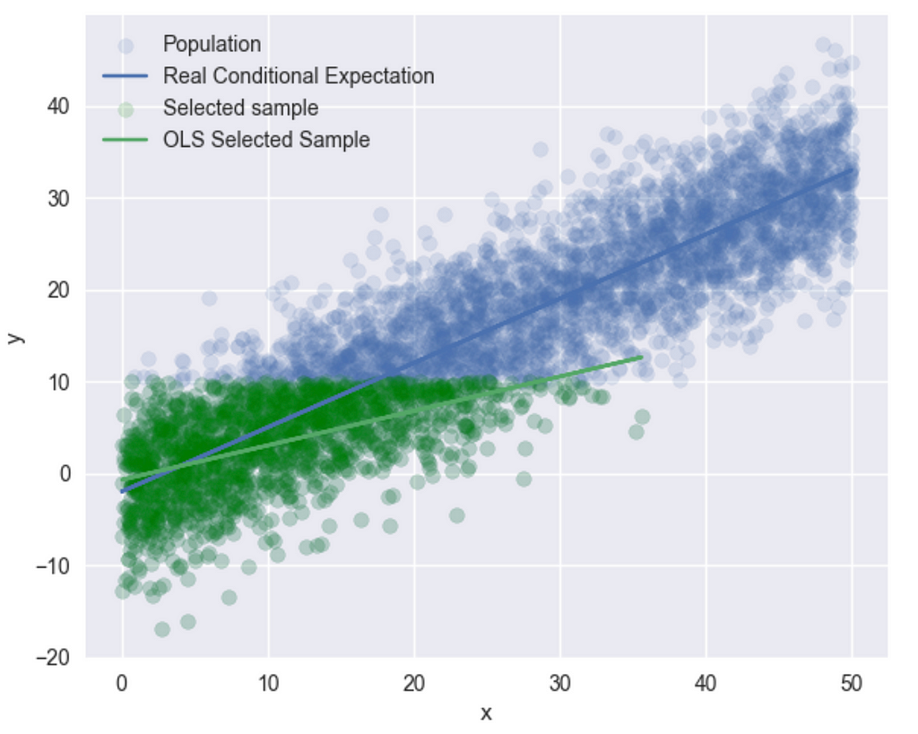
Now, OLS has provided us with a completely different line. Let’s check the correlation between the subsample X’s and the errors.

print(f"corr {np.corrcoef(df['x'], df['e'])}")
print(f"E(e|x) {np.mean(df['e'])}")

# corr [[ 1.         -0.48634973]
#  [-0.48634973  1.        ]]
# E(e|x) -2.0289245650303616

Seems like the identification assumptions are violated. Let’s also plot the sub-sample error terms, as a function of X –

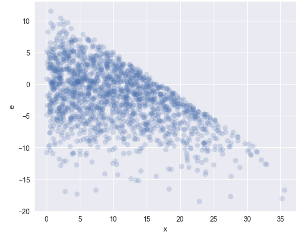
As you can see, as X increases, there are fewer large errors, indicating a clear correlation that results in biased and inconsistent OLS estimators.

Let’s explore this further.

Modeling

So, what’s going on here?

I’ll reference the model introduced by James Heckman, who, along with Daniel McFadden, received the Nobel Memorial Prize in Economic Sciences in 2000. Heckman is renowned for his pioneering work in econometrics and microeconomics, particularly for his contributions to addressing selection bias and self-selection in quantitative analysis. His well-known Heckman correction will be discussed later in this context.

In his paper from 1979, “Sample Selection Bias as a Specification Error,” Heckman illustrates how selection bias arises from censoring the dependent variable — a specific case of selection that can be extended to more non-random sample selection processes.

Censoring the dependent variable is exactly what we did when creating the last subsample in the previous section. Let’s examine Heckman’s framework.

We start with a full sample (or population) of (y_i, x_i) pairs. In this scenario, given x_i, ε_i can vary — it can be positive, negative, small, or large, depending solely on the error distribution. We refer to this complete sample of the dependent variable as y*. We then define y as the censored dependent variable, which includes only the values we actually observe.

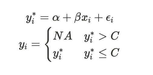
Now, let’s calculate the conditional expectation of the censored variable, y:

As you can see, this function resembles the one we saw earlier, but it includes an additional term that differs from before. This last term cannot be ignored, which means the conditional expectation function is not purely linear in terms of x (with some noise). Consequently, running OLS on the uncensored values will produce biased estimators for alpha and beta.

Moreover, this equation illustrates how the selection bias problem can be viewed as an omitted variable problem. Since the last term depends on X, it shares a significant amount of variance with the dependent variable.

Heckman’s Correction

Inverse Mills ratio

Heckman’s correction method is based on the following principle: Given a random variable Z that follows a normal distribution with mean μ and standard deviation σ, the following equations apply:

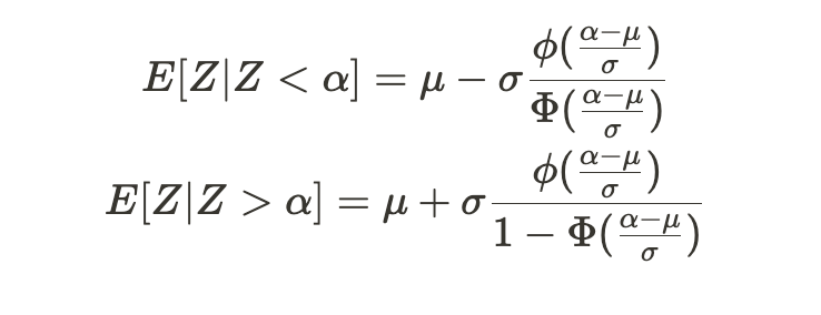
Given any constant α, Φ (capital phi) represents the standard normal distribution’s CDF, and ɸ denotes the standard normal distribution’s PDF. These values are known as the inverse Mills ratio.

So, how does this help us? Let’s revisit the last term of the previous conditional expectation equation —

Combined with the fact that our error terms follow a normal distribution, we can use the inverse Mills ratio to characterize their behavior.

Back to our model

The advantage of the inverse Mills ratio is that it transforms the previous conditional expectation function into the following form —

This results in a linear function with an additional covariate — the inverse Mills ratio. Therefore, to estimate the model parameters, we can apply OLS to this revised formula.

Let’s first calculate the inverse Mills ratio –

and in code:

from scipy.stats import norm

sample["z"] = (CENSOR-INTERCEPT-BETA*sample["x"])/SIGMA
sample["mills"] = -SIGMA*(norm.pdf(sample["z"])/(norm.cdf(sample["z"])))

and run OLS —

correcred_ols = sm.OLS(sample["y"], sm.add_constant(sample[["x", "mills"]])).fit(cov_type="HC1")
print(correcred_ols.summary())

And the output —

                            OLS Regression Results                            
==============================================================================
Dep. Variable:                      y   R-squared:                       0.313
Model:                            OLS   Adj. R-squared:                  0.313
Method:                 Least Squares   F-statistic:                     443.7
Date:                Mon, 12 Aug 2024   Prob (F-statistic):          3.49e-156
Time:                        16:47:01   Log-Likelihood:                -4840.1
No. Observations:                1727   AIC:                             9686.
Df Residuals:                    1724   BIC:                             9702.
Df Model:                           2                                         
Covariance Type:                  HC1                                         
==============================================================================
                 coef    std err          z      P>|z|      [0.025      0.975]
------------------------------------------------------------------------------
const         -1.8966      0.268     -7.088      0.000      -2.421      -1.372
x              0.7113      0.047     14.982      0.000       0.618       0.804
mills          1.0679      0.130      8.185      0.000       0.812       1.324
==============================================================================
Omnibus:                       96.991   Durbin-Watson:                   1.993
Prob(Omnibus):                  0.000   Jarque-Bera (JB):              115.676
Skew:                          -0.571   Prob(JB):                     7.61e-26
Kurtosis:                       3.550   Cond. No.                         34.7
==============================================================================

In Reality

α and β are the unobserved parameters of the model that we aim to estimate, so in practice, we cannot directly calculate the inverse Mills ratio as we did previously. Heckman introduces a preliminary step in his correction method to assist in estimating the inverse Mills ratio. This is why the Heckman’s correction is known as a two stage estimator.

To recap, our issue is that we don’t observe all the values of the dependent variable. For instance, if we’re examining how education (Z) influences wage (Y), but only observe wages above a certain threshold, we need to develop a theoretical explanation for the education levels of individuals with wages below this threshold. Once we have that, we can estimate a probit model of the following form:

and use the estimated parameters of this probit model to calculate an estimator for the inverse Mills ratio. In our case (notice I don’t use α and β) —

from statsmodels.discrete.discrete_model import Probit

pbit = Probit(df["y"] <= CENSOR, sm.add_constant(df["x"])).fit()
sample["z_pbit"] = sample["z"] = (pbit.params.const + sample["x"]*pbit.params.x)
sample["mills_pbit"] = -SIGMA*(norm.pdf(sample["z_pbit"])/(norm.cdf(sample["z_pbit"])))
correcred_ols = sm.OLS(sample["y"], sm.add_constant(sample[["x", "mills_pbit"]])).fit(cov_type="HC1")

and again, OLS for the second stage gives us consistent estimators —

                            OLS Regression Results                            
...
==============================================================================
                 coef    std err          z      P>|z|      [0.025      0.975]
------------------------------------------------------------------------------
const         -1.8854      0.267     -7.068      0.000      -2.408      -1.363
x              0.7230      0.049     14.767      0.000       0.627       0.819
mills_pbit     1.1005      0.135      8.165      0.000       0.836       1.365
==============================================================================

Wrap up

We used simulated data to demonstrate a sample selection bias problem resulting from censoring dependent variable values. We explored how this issue relates to OLS causal identification assumptions by examining the simulated errors of our model and the biased subsample. Finally, we introduced Heckman’s method for correcting the bias, allowing us to obtain consistent and unbiased estimators even when working with a biased sample.

If you enjoyed this story, I’d greatly appreciate your support — buying me a coffee would mean a lot!

References

[1] James J. Heckman, Sample Selection Bias as a Specification Error (1979), Econometrica

[2] Nick Huntington-Klein, The Effect Book (2022)

[3] Christopher Winship, Models for sample bias (1992)

Unless otherwise noted, all images are by the author

Heckman Selection Bias Modeling in Causal Studies was originally published in Towards Data Science on Medium, where people are continuing the conversation by highlighting and responding to this story.