From Data-Informed to Data-Driven Decisions: An Introduction to Tradespace Exploration

Going beyond Exploratory Data Analysis to find the needle in the haystack

DATA AND DECISIONS

The modern world is absolutely teeming with data. Empirical data, scraped and collected and stored by bots and humans alike. Artificial data, generated by models and simulations that are created and run by scientists and engineers. Even the opinions of executives and subject matter experts, recorded for later use, are data.

To what end? Why do we spend so much time and effort gathering data? The clarion call of the data revolution has been the data-driven decision: the idea that we can use this data to make better decisions. For a business, that might mean choosing the set of R&D projects or marketing pushes that will maximize future revenue. For an individual, it might simply mean an increase in satisfaction with the next car or phone or computer that they buy.

So how then do data scientists (and analysts and engineers) actually leverage their data to support decisions? Most data-to-decisions pipelines start with Exploratory Data Analysis (EDA) — the process of cleaning and characterizing a dataset, primarily using statistical analysis and supporting graphs of the spread, distribution, outliers, and correlations between the many features. EDA has many virtues that build understanding in a dataset and, by extension, any potential decision that will be made with it:

• Identifying potential errors or flawed data, and ways to correct them
• Identifying subgroups that may be under- or overrepresented in the dataset, to either be mathematically adjusted or to drive additional data collection
• Building intuition for what is possible (based on spreads) and common (based on distributions)
• Beginning to develop an understanding of potential cause-and-effect between the different features (with the permanent caveat that correlation does not equal causation)

That’s a useful first step towards a decision! A well-executed EDA will result in a reliable dataset and a set of insights about trends in the data that can be used by decision makers to inform their course of action. To overgeneralize slightly, trend insights concern the frequency of items in the dataset taking certain values: statements like “these things are usually X” or “when these things are X, these other things are usually Y”.

Unfortunately, many real-world data-to-decisions pipelines end here: taking a handful of trend insights generated by data scientists with EDA and “throwing them over the wall” to the business decision makers. The decision makers are then responsible for extrapolating these insights into the likely consequences of their (potentially many) different courses of action. Easier said than done! This is a challenging task in both complexity and scale, especially for non-technical stakeholders.

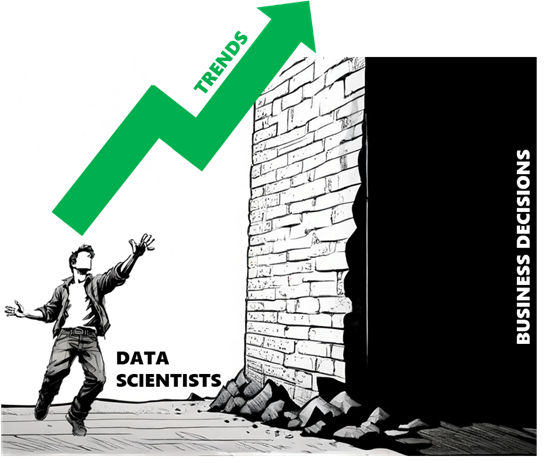
If we want to make better decisions, we need to break down that wall between the data and the decision itself. If we can collect or generate data that corresponds directly to the choices or courses of action that are available to decision makers, we can spare them the need to extrapolate from trends. Depending on the type of decision being made, this is often straightforward: like a homebuyer with a list of all the houses for sale in their area, or an engineering company with models that can evaluate thousands of potential designs for a new component.

Creating a decision-centric dataset requires a slightly different type of thinking than classic EDA, but the results are significantly easier to interpret and are therefore more likely to adequately support a decision. Instead of stopping with trends, our exploration needs to solve the needle in the haystack problem and find the best single datapoint in the set, in order to complete the data-to-decision pipeline from end-to-end.

Welcome to the world of tradespace exploration.

FROM DATA-INFORMED TO DATA-DRIVEN

Before we jump into the details of tradespace exploration, let’s ground this discussion with an example decision. Needing to buy a car is a decision many people are familiar with, and it’s a good example for a handful of reasons:

• It’s high-consequence and worth the effort to “get it right”. Cars are expensive, (ideally) last a long time, and most people use them every day! Anyone who has ever bought a lemon can tell you that it’s a particularly challenging and frustrating setback.
• People care about multiple factors when comparing cars: price, reliability, safety, handling, etc. This isn’t a problem where you can simply pick the car with the highest horsepower and expect to be satisfied.
• There are usually a lot of choices. New cars from every manufacturer, used cars from lots and online marketplaces, even things adjacent to cars like motorcycles might be valid solutions. That’s a lot of potential data to sort through!

And just to simplify this example a little bit more, let’s say that we are only interested in buying a used car.

Now, let’s think about what a normal EDA effort on this problem might look like. First, I would procure a large dataset, most commonly consisting of empirical observations: this dataset of used car sales from Craigslist [1] will do nicely. A flat data file like this one, where each item/row corresponds to a car listing described by a shared set of features/columns, is the most common format for publicly-available datasets. Then I would start with summarizing, finding problems, and cleaning the data to remove incomplete/outlier listings or inconsistently-defined columns. Once the data is clean, I would analyze the dataset with statistics or graphs to identify correlations between different variables. If you would like to see a detailed example walkthrough of EDA on this dataset, check it out here [2].

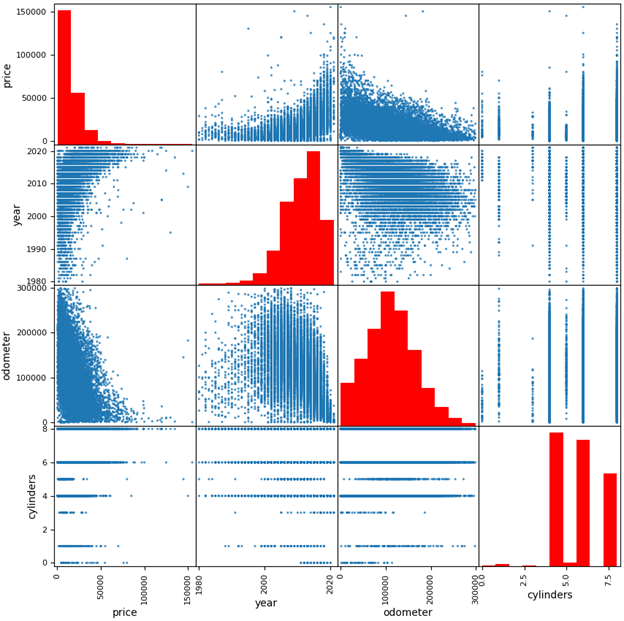
Now think about the decision again: I want to buy a used car. Did EDA help me? The good news for EDA fans and experts out there: of course it did! I’m now armed with trend insights that are highly relevant to my decision. Price is significantly correlated with model year and (negatively) with odometer mileage! Most available cars are 3–7 years old! With a greater understanding of the used car market, I will be more confident when determining if a car is a good deal or not.

But did EDA find the best car for me to buy? Not so much! I can’t actually buy the cars in the dataset since they are historical listings. If any are still active, I don’t know which ones because they aren’t indicated as such. I don’t have data on the cars that are actually available to me and therefore I still need to find those cars myself — and my EDA is useful only if the trends I found can then help me find good cars while I search a different dataset manually.

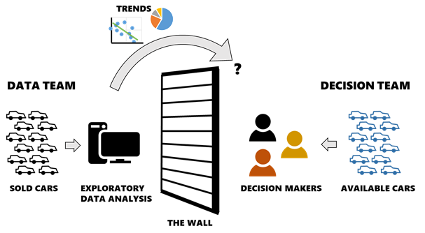
This is an example of the proverbial wall between the data and the decision, and it’s extremely common in practice because a vast majority of datasets are comprised of past/historical data but our decisions are current/future-looking. Although EDA can process a large historical dataset into a set of useful insights, there is a disconnect between the insights and the active decision because they only describe my choices by analogy (i.e. if I’m willing to assume the current used car market is similar to the past market). Perhaps it would be better to call a decision made this way data-informed rather than data-driven. A truly data-driven decision would be based on a dataset that describes the actual decision to be made — in this case, a dataset populated by currently-available car listings.

SETTING UP THE TRADESPACE

Tradespace exploration, or to be more specific Multi-Attribute Tradespace Exploration (MATE), is a framework for data-driven decision analysis. Originally created at MIT in 2000, it has undergone decades of refinement and application through today [3–7]. MATE brings value-focused thinking [8] to the world of large datasets, with the express purpose of increasing the value created by decisions being made with that data.

The MATE framework helps decision makers and data scientists/analysts think critically about how to define and structure a decision problem, how to perform data collection, and finally how to explore that data to generate practical, relevant insights and find the best solution. At a high level, MATE is broken into three layers corresponding to these steps: Define, Generate, and Explore.

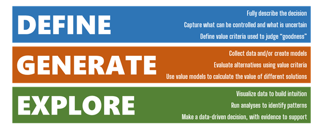
Defining a basic MATE study begins with a few core concepts:

• Stakeholders. Who makes the decision or is affected by it? For simplicity, let’s say that I’m the only stakeholder for my car purchase; however, keep in mind that many decisions have multiple stakeholders with potentially very different needs and desires and we can and should consider them all.
• Alternatives. What are the possible solutions, i.e. what are the available choices? I already restricted myself to buying a used car in this example. My alternatives are any used cars that are available for sale within a reasonable distance of where I live. Importantly, alternatives should be unique: I can define my choices with fundamental variables like manufacturer, model, and year, but a unique identifier like their VIN is also necessary in case there are multiple listings of the same car type.
• Resources. How do the stakeholders acquire and use an alternative, i.e. what needs to be spent? Each car will have a one-time purchase price. I could also choose to consider ownership costs that are incurred later on such as fuel and maintenance, but we’ll ignore these for now.
• Benefits. Why do we want an alternative, i.e. what criteria do the stakeholders use to judge how “good” an alternative is? Maybe I care about the number of passengers a car can carry (for practicality), its engine cylinders (for fun), its odometer mileage (for longevity), and its safety rating (for… safety).

This simple outline gives us direction on how to then collect data during the Generate step. In order to properly capture this decision, I need to collect data for all of the alternative variables, resources, and benefits that I identified in the Define step. Anything less would give me an incomplete picture of value — but I can always include any additional variables that I think are informative.

Imagine for a moment that the Craigslist cars dataset DID include a column that indicated which listings were still available for purchase, and therefore are real alternatives for my decision. Am I done collecting data? No — this dataset includes my alternative variables (manufacturer, model, year, VIN) and my resources (price) but is missing two of my benefits: passenger count and safety rating. I will need to supplement this dataset with additional data, or I won’t be able to accurately judge how much I like each car. This requires some legwork on the part of the analyst to source the new data and properly match it up with the existing dataset in new columns.

Fortunately, the alternative variables can act as “keys” to cross-reference different datasets. For example, I need to find a safety rating for each alternative. Safety ratings are generally given to a make/model/year of car, so I can either:

• Find tabular data on safety ratings (compiled by someone else), and combine it with my own data by joining the tables on the columns make/model/year
• Collect safety rating data myself and plug it directly into my table, for example by searching https://www.nhtsa.gov/ratings for each alternative using its make/model/year

I may also want to supplement the Craigslist data with additional alternatives: after all, not all used cars are for sale on Craigslist. It is considered best practice for MATE to start with as large a set of alternatives as possible, to not preemptively constrain the decision. By going to the websites of nearby car dealerships and searching for their used inventory, I can add more cars to my dataset as additional rows. Depending on how many cars are available (and my own motivation), I could possibly even automate this process with a web scraper, which is how data collection is often performed at-scale. Remember though: I still need to have data for at least the alternative variables, resources, and benefits for each car in the dataset. Most dealership listings won’t include details like safety ratings, so I will need to supplement these with other data sources in the same way as before.

At this point, I have my data “haystack” and I’m almost ready to start the Explore layer and look for that “needle”. But what do I do? How does MATE really differ from our old friend EDA?

WHAT MAKES A GOOD SOLUTION?

Now that I have my dataset populated with relevant alternatives for my actual decision, could I just perform EDA on it to solve the problem and find the best car? Well… yes and no. You can (and should!) perform EDA on a MATE dataset — cleaning potential errors or weirdness out of the dataset remains relevant and is especially important if data was collected via an automated process like a web scraper. And the goals of building intuition for trends in the data are no different: the better we understand how different criteria are related, the more confident we will become in our eventual decision. For example, the scatterplot matrix I showed a few pictures ago is also a common visualization for MATE.

But even with a dataset of active car listings and all the necessary variables, the bread-and-butter correlation and distribution analyses of EDA don’t help to pull out individual high-value datapoints. Remember: we care about lots of different properties of a car (the multi-attributes of Multi-Attribute Tradespace Exploration), so we can’t simply sort by price and take the cheapest car. Armed with just EDA trend insights, I’m still going to need to manually check a lot of potential choices until I find a car with a desirable combination of features and performance and price.

What I need is a tool to pull the best cars to the top of the pile. That tool: value modeling.

At the most basic level, a value model is a mathematical function that attempts to replicate the preferences of a stakeholder. We feed the benefits and/or resources identified in the Define layer in, and get out a value score that says how “good” each alternative is. If the model is accurate, our stakeholder will prefer an alternative (car) over any other with a lower score. [9]

Most data scientists have probably created and used a simple value model many times (whether or not they realized it or called it by a different name), as a means of doing exactly this task: creating a new column in a dataset that “scores” the rows with a function of the other columns, so that the dataset could be sorted and high-scoring rows highlighted. There are many different types of value models, each with its own strengths and weaknesses. More accurate value models are generally more complex and correspondingly take more effort to create.

For this example, we will use a simplified utility function to combine the four benefits I stand to gain from buying a car [10]. There is a formal elicitation process that can be completed with the stakeholder (me) to create a verifiably correct utility function, but we’ll just construct one quickly by assigning each attribute a threshold requirement (worst-acceptable level), objective (maximally-valuable level, no extra value for outperforming this point), and swing weight (a measure of importance). There are other ways to customize a utility function, including non-linear curves and complementarity/substitution effects that we will skip this time.

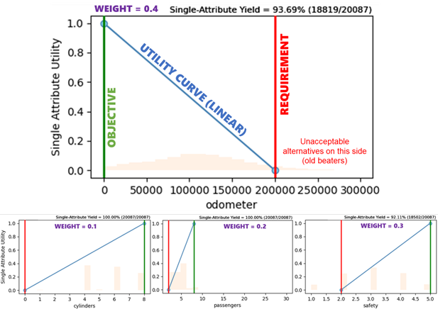
But wait: why didn’t I include price in the utility function? The technical answer is that most people display “incomplete ordering” [11] between benefits and resources — a fancy way of saying that stakeholders will often be unable to definitively state whether they prefer a low-cost-low-benefit alternative or a high-cost-high-benefit alternative since neither is strictly superior to the other. Incidentally, this is also why it is very difficult to “solve” a decision by optimizing a function: in practice, decision makers generally like to see a set of alternatives that vary from low-cost-low-benefit to high-cost-high-benefit and judge for themselves, and this ends up being more reliable than combining benefits/costs into one value model. This set is called the Pareto set (or Pareto front, when viewed graphically), and is the highest-value region of the tradespace.

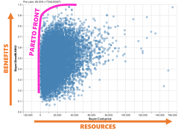
And here we have it: “the tradespace”. A scatterplot with benefit on the y-axis and cost on the x-axis (each potentially a value model composed of multiple attributes). A tradeoff between benefits and costs is by far the most common real-world-plain-English framing of a decision, and the MATE framework exists to guide the data-driven analysis of our decisions into this structure that stakeholders and decision makers are familiar with. Each one of those points is a car I could buy — a choice I can actually make, and a way to solve my decision without relying on extrapolation from past trends.

All that’s left now is the Explore layer, where I need to find my favorite needle from among that haystack of points.

FINDING THE NEEDLE

Let’s do a quick exploring session on my cars dataset using EpochShift, a program for creating and exploring MATE datasets (full disclosure: I am currently working on EpochShift’s development, but you can replicate these plots with some time and elbow grease in the visualization library of your choice). First, because they are likely candidates for me to buy, I’m going to highlight the cars in the Pareto set with a blaze — a custom marker that appears “on top” of the plot, and persists even if I change the plot dimensions. I’m also curious about the relationship that odometer mileage has with the value dimensions of the tradespace, so I will color the points using that parameter.

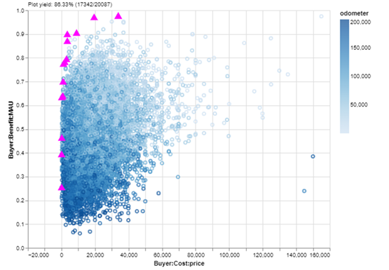
Two issues pop out at me right away:

• It’s a little tough to discern a pattern in odometer mileage because the tradespace of 17,000+ cars is so dense that the points occlude each other: some points cover up others. I can tell that the points generally fade from dark to light moving up the y-axis, but if I could remove the occlusion, I could more clearly see the spread of different tiers of mileage on my benefit/resource dimensions.
• I also can’t tell the odometer mileage of the cars in the Pareto set because they are magenta. If I could still highlight those while also seeing their mileage color, that would be ideal.

To address these, I’ll modify my plot in two ways:

• I’ll replace the points in the tradespace with convex hulls — essentially dividing the range of odometer mileage into smaller chunks and drawing a “bubble” around all the cars in each chunk.
• I’ll leave my Pareto set blaze in place, but update it to have the triangle filled with the corresponding odometer mileage color.

With those two changes, I get this:

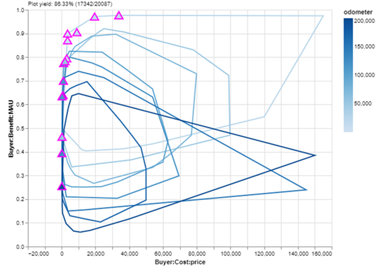
Look at that! I can see a clear relationship between odometer mileage and utility, which makes sense since that was one of the benefit metrics I used in my value model. Additionally, with the exception of a couple (delusional) sellers in the lower-right of the plot, it’s clear that cars with higher mileage have a lower top-end asking price — but perhaps more interestingly, mileage does not seem to strongly impact low-end asking prices. Even low mileage cars are available for cheap!

But let’s get back to making a decision by focusing on the Pareto set. I didn’t screen the dataset to remove high-cost cars because, as I mentioned before, it’s considered MATE best practice not to reduce the number of alternatives before beginning the Explore layer. But realistically, I have a budget for this purchase of $10K, and maybe I want the best car available under that limit — especially now that I know I’ll still be able to find a car with low mileage in that price range. I’ll add my budget requirement and switch back to a scatterplot:

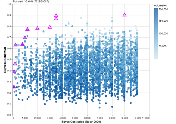
Okay, now we are looking at a nice zoom-in of affordable cars. If I just want to buy the car with the most benefit in my budget, it will be the Pareto set point farthest up and to the right. I can check the details of that car with a mouseover:

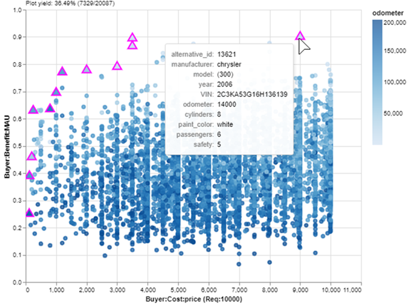
A 2006 Chrysler 300 with 14,000 miles for $9K. Not too bad! But wait… it’s painted white. I forgot that I hate white cars! Part of the Explore layer of MATE is refining stakeholder preferences, which often change when exposed to new information: the data of my data-driven decision. One advantage of using an interactive tool is that I can easily update value models or filters in response to these changes. I’ll just add a filter that removes white cars, save a new Pareto set and:

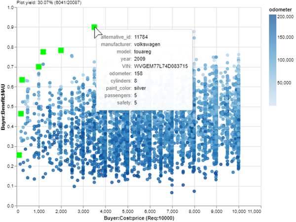
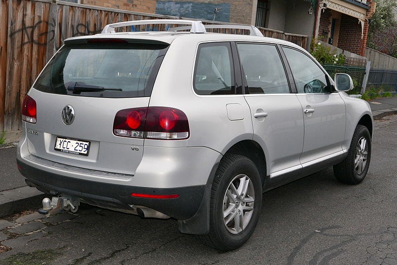
There! Now the best car in my budget is a silver 2009 Volkswagen Touareg. I lost one passenger compared to the Chrysler (6 to 5) which is not ideal, but the utility of this car is nearly as high thanks to its significantly lower odometer (14,000 to 158). It’s practically new and it only costs $3500!

We found it: the needle in the haystack. And we can justify our decision with data-driven evidence!

CONCLUSION

The goal of this article was to show how EDA and tradespace exploration are similar/complementary but highlight a few key differences in how data is collected and visualized when the end goal is to find the “best” point in a dataset. Tradespace exploration can be the “one step beyond” EDA that pushes a decision from data-informed to truly data-driven. But this short example only scratches the surface of what we can do with MATE.

The MATE framework supports many additional types of data and analysis. More complex and/or important decisions may require these features for you (or your stakeholders) to feel confident that the best decision has been reached:

• Including multiple stakeholders, each with their own value models, and the search for solutions that are desirable and equitable for all parties
• Including uncertainty, resulting in multiple scenarios (each with its own tradespace), and the search for solutions that are robust to unknown or uncontrollable parameters
• Adding dynamics and options, allowing the scenario to change repeatedly over time while we responsively modify our solution to maximize value
• Many new and interesting visualizations to support the analysis of these complex problems

If this piqued your interest and you want to learn more about tradespace exploration, follow me or The Tradespace on Medium, where we are working to teach people of all skill levels how to best apply MATE to their problems. Or feel free to reach out via email/comment if you have any questions or cool insights — I hope to hear from you!

REFERENCES

[1] A. Reese, Used Cars Dataset (2021), https://www.kaggle.com/datasets/austinreese/craigslist-carstrucks-data

[2] T. Shin, An Extensive Step by Step Guide to Exploratory Data Analysis (2020), Towards Data Science.

[3] A. Ross, N. Diller, D. Hastings, and J. Warmkessel, Multi-Attribute Tradespace Exploration in Space System Design (2002), IAF IAC-02-U.3.03, 53rd International Astronautical Congress — The World Space Congress, Houston, TX.

[4] A. Ross and D. Hastings, The Tradespace Exploration Paradigm (2005), INCOSE International Symposium 2005, Rochester, NY.

[5] M. Richards, A. Ross, N. Shah, and D. Hastings, Metrics for Evaluating Survivability in Dynamic Multi-Attribute Tradespace Exploration (2009), Journal of Spacecraft and Rockets, Vol. 46, №5, September-October 2009.

[6] M. Fitzgerald and A. Ross, Recommendations for Framing Multi-Stakeholder Tradespace Exploration (2016), INCOSE International Symposium 2016, Edinburgh, Scotland, July 2016.

[7] C. Rehn, S. Pettersen, J. Garcia, P. Brett, S. Erikstad, B. Asbjornslett, A. Ross, and D. Rhodes, Quantification of Changeability Level for Engineering Systems (2019), Systems Engineering, Vol. 22, №1, pp. 80–94, January 2019.

[8] R. Keeney, Value-Focused Thinking: A Path to Creative Decision-Making (1992). Harvard University Press, Cambridge.

[9] N. Ricci, M. Schaffner, A. Ross, D. Rhodes, and M. Fitzgerald, Exploring Stakeholder Value Models Via Interactive Visualization (2014), 12th Conference on Systems Engineering Research, Redondo Beach, CA, March 2014.

[10] R. Keeney and H. Raiffa, Decisions with Multiple Objectives: Preferences and Value Trade-Offs (1993), Cambridge University Press.

[11] J. Von Neumann and O. Morgenstern, Theory of games and economic behavior (1944), Princeton University Press.

From Data-Informed to Data-Driven Decisions: An Introduction to Tradespace Exploration was originally published in Towards Data Science on Medium, where people are continuing the conversation by highlighting and responding to this story.