
How integrating Batch Normalization in an encoder-only Transformer architecture can lead to reduced training time and inference time.

Introduction
The introduction of transformer-based architectures, pioneered by the discovery of the Vision Transformer (ViT), has ushered in a revolution in the field of Computer Vision. For a wide range of applications, ViT and its various cousins have effectively challenged the status of Convolutional Neural Networks (CNNs) as the state-of-the-art architecture (see this paper for a nice comparative study). Yet, in spite of this success, ViTs are known to require significantly longer training times and have slower inference speed for smaller-to-medium input data sizes. It is therefore an important issue to study modifications of the Vision Transformer which may lead to faster training and inference speeds.
In this first article of a three-part series, I explore in detail one such modification of the ViT, which will involve replacing Layer Normalization (LayerNorm) — the default normalization technique for transformers — with Batch Normalization (BatchNorm). More specifically, I will discuss two versions of such a model. As I will review in a minute, the ViT has an encoder-only architecture with the transformer encoder consisting of two distinct modules — the multi-headed self-attention (MHSA) and the feedforward network (FFN). The first model will involve implementing a BatchNorm layer only in the feedforward network — this will be referred to as ViTBNFFN (Vision Transformer with BatchNorm in the feedforward network). The second model will involve replacing the LayerNorm with BatchNorm everywhere in the Vision Transformer — I refer to this model as ViTBN (Vision Transformer with BatchNorm). Therefore, the model ViTBNFFN will involve both LayerNorm (in the MHSA) and BatchNorm (in the FFN), while ViTBN will involve BatchNorm only.
I will compare the performances of the three models — ViTBNFFN, ViTBN and the standard ViT — on the MNIST dataset of handwritten digits. To be more specific, I will compare the following metrics— training time per epoch, testing/inference time per epoch, training loss and test accuracy for the models in two distinct experimental set-ups. In the first set-up, the models are compared at a fixed choice of hyperparameters (learning rate and batch size). The exercise is then repeated at different values of the learning rate keeping all the other hyperparameters (like batch size) unchanged. In the second set-up, one first finds the best choice of hyperparamters for each model that maximizes the accuracy using a Bayesian Optimization procedure. The performances of these optimized models are then compared in terms of the metrics mentioned above. I find that in both set-ups, the models ViTBNFFN and ViTBN lead to more than 60% gain in the average training time per epoch as well as the average inference time per epoch while giving a comparable (or superior) accuracy compared to the standard ViT. In addition, the models with BatchNorm allow for a larger learning rate compared to ViT without compromising the stability of the models. The latter finding is consistent with the general intuition of BatchNorm deployed in CNNs, as pointed out in the original paper of Ioffe and Szegedy.
In the second article of the series, I compare the performances of the three trained models on a different dataset — the EMNIST (Extended MNIST) dataset of handwritten digits. To obtain the trained models, I first introduce certain image augmentations in the MNIST data and perform a Bayesian Optimization to obtain the best set of hyperparameters for each model. The optimized models are then trained for an equal number of epochs on the augmented MNIST data. I then compare the performances of these models on the EMNIST dataset in terms of inference time per epoch and accuracy. In this case too, I find that the models with BatchNorm register a significant gain in the inference times. As an order of magnitude estimate, I compare the inference times of these models with that of a CNN model trained on the same data.
In the third and final article, I use the best performing Vision Transformer model with BatchNorm to build a Flask-based app for recognizing digits that a user draws using a touchpad. I then discuss how to deploy the app on the web with the pythonanywhere platform as well as to AWS Elastic Beanstalk using Docker.
You can fork the code used in these articles at the github repo and play around with it. Let me know what you think!
Contents
I begin with a gentle introduction to BatchNorm and its PyTorch implementation followed by a brief review of the Vision Transformer. Readers familiar with these topics can skip to the next section, where we describe the implementation of the ViTBNFFN and the ViTBN models using PyTorch. Next, I set up the simple numerical experiments using the tracking feature of MLFlow to train and test these models on the MNIST dataset (without any image augmentation), and compare the results with those of the standard ViT. The Bayesian optimization is performed using the BoTorch optimization engine available on the Ax platform. I end with a brief summary of the results and a few concluding remarks.
Batch Normalization : Definition and PyTorch Implementation
Let us briefly review the basic concept of BatchNorm in a deep neural network. The idea was first introduced in a paper by Ioffe and Szegedy as a method to speed up training in Convolutional Neural Networks. Suppose zᵃᵢ denote the input for a given layer of a deep neural network, where a is the batch index which runs from a=1,…, Nₛ and i is the feature index running from i=1,…, C. Here Nₛ is the number of samples in a batch and C is the dimension of the layer that generates zᵃᵢ. The BatchNorm operation then involves the following steps:
- For a given feature i, compute the mean and the variance over the batch of size Nₛ i.e.

2. For a given feature i, normalize the input using the mean and variance computed above, i.e. define ( for a fixed small positive number ϵ):

3. Finally, shift and rescale the normalized input for every feature i:

where there is no summation over the indices a or i, and the parameters (γᵃᵢ, βᵃᵢ) are trainable.
The layer normalization (LayerNorm) on the other hand involves computing the mean and the variance over the feature index for a fixed batch index a, followed by analogous normalization and shift-rescaling operations.
PyTorch has an in-built class BatchNorm1d which performs batch normalization for a 2d or a 3d input with the following specifications:
In a generic image processing task, an image is usually divided into a number of smaller patches. The input z then has an index α (in addition to the indices a and i) which labels the specific patch in a sequence of patches that constitutes an image. The BatchNorm1d class treats the first index of the input as the batch index and the second as the feature index, where num_features = C. It is therefore important that the input is a 3d tensor of the shape Nₛ × C × N where N is the number of patches. The output tensor has the same shape as the input. PyTorch also has a class BatchNorm2d that can handle a 4d input. For our purposes it will be sufficient to make use of the BatchNorm1d class.
The BatchNorm1d class in PyTorch has an additional feature that we need to discuss. If one sets track_running_stats = True (which is the default setting), the BatchNorm layer keeps running estimates of its computed mean and variance during training (see here for more details), which are then used for normalization during testing. If one sets the option track_running_stats = False, the BatchNorm layer does not keep running estimates and instead uses the batch statistics for normalization during testing as well. For a generic dataset, the default setting might lead to the training and the testing accuracies being significantly different, at least for the first few epochs. However, for the datasets that I work with, one can explicitly check that this is not the case. I therefore simply keep the default setting while using the BatchNorm1d class.
The Standard Vision Transformer : A Brief Review
The Vision Transformer (ViT) was introduced in the paper An Image is worth 16 × 16 words for image classification tasks. Let us begin with a brief review of the model (see here for a PyTorch implementation). The details of the architecture for this encoder-only transformer model is shown in Figure 1 below, and consists of three main parts: the embedding layers, a transformer encoder, and an MLP head.
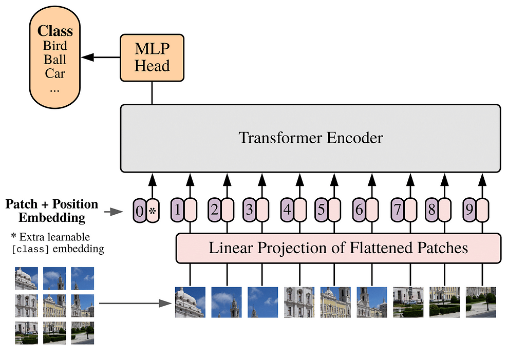
The embedding layers break up an image into a number of patches and maps each patch to a vector. The embedding layers are organized as follows. One can think of a 2d image as a real 3d tensor of shape H× W × c with H,W, and c being the height, width (in pixels) and the number of color channels of the image respectively. In the first step, such an image is reshaped into a 2d tensor of shape N × dₚ using patches of size p, where N= (H/p) × (W/p) is the number of patches and dₚ = p² × c is the patch dimension. As a concrete example, consider a 28 × 28 grey-scale image. In this case, H=W=28 while c=1. If we choose a patch size p=7, then the image is divided into a sequence of N=4 × 4 = 16 patches with patch dimension dₚ = 49.
In the next step, a linear layer maps the tensor of shape N × dₚ to a tensor of shape N × dₑ , where dₑ is known as the embedding dimension. The tensor of shape N × dₑ is then promoted to a tensor y of shape (N+1) × dₑ by prepending the former with a learnable dₑ-dimensional vector y₀. The vector y₀ represents the embedding of CLS tokens in the context of image classification as we will explain below. To the tensor y one then adds another tensor yₑ of shape (N+1) × dₑ — this tensor encodes the positional embedding information for the image. One can either choose a learnable yₑ or use a fixed 1d sinusoidal representation (see the paper for more details). The tensor z = y + yₑ of shape (N+1) × dₑ is then fed to the transformer encoder. Generically, the image will also be labelled by a batch index. The output of the embedding layer is therefore a 3d tensor of shape Nₛ × (N+1) × dₑ.
The transformer encoder, which is shown in Figure 2 below, takes a 3d tensor zᵢ of shape Nₛ × (N+1) × dₑ as input and outputs a tensor zₒ of the same shape. This tensor zₒ is in turn fed to the MLP head for the final classification in the following fashion. Let z⁰ₒ be the tensor of shape Nₛ × dₑ corresponding to the first component of zₒ along the second dimension. This tensor is the “final state” of the learnable tensor y₀ that prepended the input tensor to the encoder, as I described earlier. If one chooses to use CLS tokens for the classification, the MLP head isolates z⁰ₒ from the output zₒ of the transformer encoder and maps the former to an Nₛ × n tensor where n is the number of classes in the problem. Alternatively, one may also choose perform a global pooling whereby one computes the average of the output tensor zₒ over the (N+1) patches for a given feature which results in a tensor zᵐₒ of shape Nₛ × dₑ. The MLP head then maps zᵐₒ to a 2d tensor of shape Nₛ × n as before.
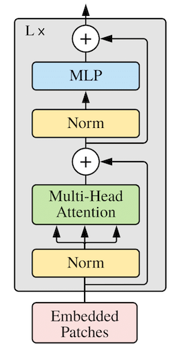
Let us now discuss the constituents of the transformer encoder in more detail. As shown in Figure 2, it consists of L transformer blocks, where the number L is often referred to as the depth of the model. Each transformer block in turn consists of a multi-headed self attention (MHSA) module and an MLP module (also referred to as a feedforward network) with residual connections as shown in the figure. The MLP module consists of two hidden layers with a GELU activation layer in the middle. The first hidden layer is also preceded by a LayerNorm operation.
We are now prepared to discuss the models ViTBNFFN and ViTBN.
Vision Transformer with BatchNorm : ViTBNFFN and ViTBN
To implement BatchNorm in the ViT architecture, I first introduce a new BatchNorm class tailored to our task:
This new class Batch_Norm uses the BatchNorm1d (line 10) class which I reviewed above. The important modification appears in the lines 13–15. Recall that the input tensor to the transformer encoder has the shape Nₛ × (N+1) × dₑ. At a generic layer inside the encoder, the input is a 3d tensor with the shape Nₛ × (N+1) × D, where D is the number of features at that layer. For using the BatchNorm1d class, one has to reshape this tensor to Nₛ × D × (N+1), as we explained earlier. After implementing the BatchNorm, one needs to reshape the tensor back to the shape Nₛ × (N+1) × D, so that the rest of the architecture can be left untouched. Both reshaping operations are done using the function rearrange which is part of the einops package.
One can now describe the models with BatchNorm in the following fashion. First, one may modify the feedforward network in the transformer encoder of the ViT by removing the LayerNorm operation that precedes the first hidden layer and introducing a BatchNorm layer. I will choose to insert the BatchNorm layer between the first hidden layer and the GELU activation layer. This gives the model ViTBNFFN. The PyTorch implementation of the new feedforward network is given as follows:
The constructor of the FeedForward class, given by the code in the lines 7–11, is self-evident. The BatchNorm layer is being implemented by the Batch_Norm class in line 8. The input tensor to the feedforward network has the shape Nₛ × (N+1) × dₑ. The first linear layer transforms this to a tensor of shape Nₛ × (N+1) × D, where D= hidden_dim (which is also called the mlp_dimension) in the code. The appropriate feature dimension for the Batch_Norm class is therefore D.
Next, one can replace all the LayerNorm operations in the model ViTBNFFN with BatchNorm operations implemented by the class Batch_Norm. This gives the ViTBN model. We make a couple of additional tweaks in ViTBNFFN/ViTBN compared to the standard ViT. Firstly, we incorporate the option of having either a learnable positional encoding or a fixed sinusoidal one by introducing an additional model parameter. Similar to the standard ViT, one can choose a method involving either CLS tokens or global pooling for the final classification. In addition, we replace the MLP head by a simpler linear head. With these changes, the ViTBN class assumes the following form (the ViTBNFFN class has an analogous form):
Most of the above code is self-explanatory and closely resembles the standard ViT class. Firstly, note that in the lines 23–28, we have replaced LayerNorm with BatchNorm in the embedding layers. Similar replacements have been performed inside the Transformer class representing the transformer encoder that ViTBN uses (see line 44). Next, we have added a new hyperparameter “pos_emb” which takes as values the string ‘pe1d’ or ‘learn’. In the first case, one uses the fixed 1d sinusoidal positional embedding while in the second case one uses learnable positional embedding. In the forward function, the first option is implemented in the lines 62–66 while the second is implemented in the lines 68–72. The hyperparameter “pool” takes as values the strings ‘cls’ or ‘mean’ which correspond to a CLS token or a global pooling for the final classification respectively. The ViTBNFFN class can be written down in an analogous fashion.
The model ViTBN (analogously ViTBNFFN) can be used as follows:
In this specific case, we have the input dimension image_size = 28 which implies H = W = 28. The patch_size = p =7 means that the number of patches are N= 16. With the number of color channels being 1, the patch dimension is dₚ =p²= 49. The number of classes in the classification problem is given by num_classes. The parameter dim= 64 in the model is the embedding dimension dₑ . The number of transformer blocks in the encoder is given by the depth = L =6. The parameters heads and dim_head correspond to the number of self-attention heads and the (common) dimension of each head in the MHSA module of the encoder. The parameter mlp_dim is the hidden dimension of the MLP or feedforward module. The parameter dropout is the single dropout parameter for the transformer encoder appearing both in the MHSA as well as in the MLP module, while emb_dropout is the dropout parameter associated with the embedding layers.
Experiment 1: Comparing Models at Fixed Hyperparameters
Having introduced the models with BatchNorm, I will now set up the first numerical experiment. It is well known that BatchNorm makes deep neural networks converge faster and thereby speeds up training and inference. It also allows one to train CNNs with a relatively large learning rate without bringing in instabilities. In addition, it is expected to act as a regularizer eliminating the need for dropout. The main motivation of this experiment is to understand how some of these statements translate to the Vision Transformer with BatchNorm. The experiment involves the following steps :
- For a given learning rate, I will train the models ViT, ViTBNFFN and ViTBN on the MNIST dataset of handwritten images, for a total of 30 epochs. At this stage, I do not use any image augmentation. I will test the model once on the validation data after each epoch of training.
- For a given model and a given learning rate, I will measure the following quantities in a given epoch: the training time, the training loss, the testing time, and the testing accuracy. For a fixed learning rate, this will generate four graphs, where each graph plots one of these four quantities as a function of epochs for the three models. These graphs can then be used to compare the performance of the models. In particular, I want to compare the training and the testing times of the standard ViT with that of the models with BatchNorm to check if there is any significant speeding up in either case.
- I will perform the operations in Step 1 and Step 2 for three representative learning rates l = 0.0005, 0.005 and 0.01, holding all the other hyperparameters fixed.
Throughout the analysis, I will use CrossEntropyLoss() as the loss function and the Adam optimizer, with the training and testing batch sizes being fixed at 100 and 5000 respectively for all the epochs. I will set all the dropout parameters to zero for this experiment. I will also not consider any learning rate decay to keep things simple. The other hyperparameters are given in Code Block 5 — we will use CLS tokens for classification which corresponds to setting pool = ‘cls’ , and learnable positional embedding which corresponds to setting pos_emb = ‘learn’.
The experiment has been conducted using the tracking feature of MLFlow. For all the runs in this experiment, I have used the NVIDIA L4 Tensor Core GPU available at Google Colab.
Let us begin by discussing the important ingredients of the MLFlow module which we execute for a given run in the experiment. The first of these is the function train_model which will be used for training and testing the models for a given choice of hyperparameters:
The function train_model returns four quantities for every epoch — the training loss (cost_list), test accuracy (accuracy_list), training time in seconds (dur_list_train) and testing time in seconds (dur_list_val). The lines of code 19–32 give the training module of the function, while the lines 35–45 give the testing module. Note that the function allows for testing the model once after every epoch of training. In the Git version of our code, you will also find accuracies by class, but I will skip that here for the sake of brevity.
Next, one needs to define a function that will download the MNIST data, split it into the training dataset and the validation dataset, and transform the images to torch tensors (without any augmentation):
We are now prepared to write down the MLFlow module which has the following form:
Let us explain some of the important parts of the code.
- The lines 11–13 specify the learning rate, the number of epochs and the loss function respectively.
- The lines 16–33 specify the various details of the training and testing. The function get_datesets() of Code Block 7 downloads the training and validation datasets for the MNIST digits, while the function get_model() defined in Code Block 5 specifies the model. For the latter, we set pool = ‘cls’ , and pos_emb = ‘learn’. On line 20, the optimizer is defined, and we specify the training and validation data loaders including the respective batch sizes on lines 21–24. Line 25–26 specifies the output of the function train_model that we have in Code Block 6— four lists each with n_epoch entries. Lines 16–24 specify the various arguments of the function train_model.
- On lines 37–40, one specifies the parameters that will be logged for a given run of the experiment, which for our experiment are the learning parameter and the number of epochs.
- Lines 44–52 constitute the most important part of the code where one specifies the metrics to be logged i.e. the four lists mentioned above. It turns out that by default the function mlflow.log_metrics() does not log a list. In other words, if we simply use mlflow.log_metrics({generic_list}), then the experiment will only log the output for the last epoch. As a workaround, we call the function multiple times using a for loop as shown.
Let us now take a deep dive into the results of the experiment, which are essentially summarized in the three sets of graphs of Figures 3–5 below. Each figure presents a set of four graphs corresponding to the training time per epoch (top left), testing time per epoch (top right), training loss (bottom left) and test accuracy (bottom right) for a fixed learning rate for the three models. Figures 3, 4 and 5 correspond to the learning rates l=0.0005, l=0.005 and l=0.01 respectively. It will be convenient to define a pair of ratios :

where T(model|train) and T(model|test) are the average training and testing times per epoch for given a model in our experiment. These ratios give a rough measure of the speeding up of the Vision Transformer due to the integration of BatchNorm. We will always train and test the models for the same number of epochs — one can therefore define the percentage gains for the average training and testing times per epoch in terms of the above ratios respectively as:

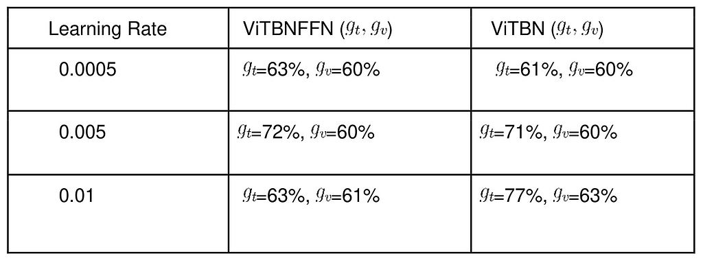
Let us begin with the smallest learning rate l=0.0005 which corresponds to Figure 3. In this case, the standard ViT converges in a fewer number of epochs compared to the other models. After 30 epochs, the standard ViT has lower training loss and marginally higher accuracy (~ 98.2 %) compared to both ViTBNFFN (~ 97.8 %) and ViTBN (~ 97.1 %) — see the bottom right graph. However, the training time and the testing time are higher for ViT compared to ViTBNFFN/ViTBN by a factor greater than 2. From the graphs, one can read off the ratios rₜ and rᵥ : rₜ (ViTBNFFN) = 2.7 , rᵥ (ViTBNFFN)= 2.6, rₜ (ViTBNFFN) = 2.5, and rᵥ (ViTBN)= 2.5 , where rₜ , rᵥ have been defined above. Therefore, for the given learning rate, the gain in speed due to BatchNorm is significant for both training and inference — it is roughly of the order of 60%. The precise percentage gains are listed in Table 1.
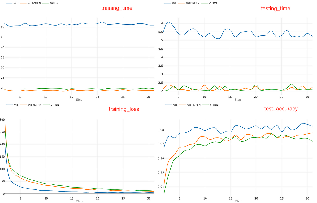
In the next step, we increase the learning rate to l=0.005 and repeat the experiment, which yields the set of graphs in Figure 4.
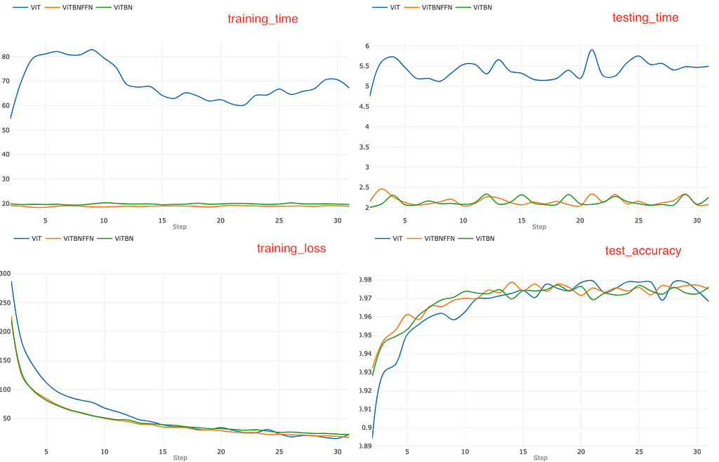
For a learning rate l=0.005, the standard ViT does not seem to have any advantage in terms of faster convergence. However, the training time and the testing time are again higher for ViT compared to ViTBNFFN/ViTBN. A visual comparison of the top left graphs in Figure 3 and Figure 4 indicates that the training time for ViT increases significantly while those for ViTBNFFN and ViTBN roughly remain the same. This implies that there is a more significant gain in training time in this case. On the other hand, comparing the top right graphs in Figure 3 and Figure 4, one can see that gain in testing speed is roughly the same. The ratios rₜ and rᵥ can again be read off from the top row of graphs in Figure 4 : rₜ (ViTBNFFN) = 3.6 , rᵥ (ViTBNFFN)=2.5, rₜ (ViTBN) = 3.5 and rᵥ (ViTBN)= 2.5. Evidently, the ratios rₜ are larger here compared to the case with smaller learning rate, while the ratios rᵥ remain about the same. This leads to a higher percentage gain (~70%) in training time, with the gain for inference time (~60%) remaining roughly the same.
Finally, let us increase the learning rate even further to l=0.01 and repeat the experiment, which yields the set of graphs in Figure 5.

In this case, ViT becomes unstable after a few epochs as one can see from the training_loss graph in Figure 5, which shows a non-converging behavior starting in the vicinity of epoch 15. This is also corroborated by the test_accuracy graph where the accuracy of ViT can be seen to plummet around epoch 15. However, the models ViTBNFFN and ViTBN remain stable and reach accuracies higher than 97% at the end of 30 epochs of training. The training time for ViT is even higher in this case and fluctuates wildly. For ViTBNFFN, there is an appreciable increase in the training time, while it remains roughly the same for ViTBN — see the top left graph. In terms of the training ratios rₜ, we have rₜ (ViTBNFFN) = 2.7 and rₜ(ViTBN)=4.3. The first ratio is lower than what we found in the previous case. This is an artifact of the higher training time for ViTBNFFN, which offsets the increase in the training time for ViT. The second ratio is significantly higher since the training time for ViTBN roughly remains unchanged. The test ratios rᵥ in this case — rᵥ (ViTBNFFN)=2.6 and rᵥ (ViTBN)= 2.7 — show a tiny increase.
The gains in training and inference times — gₜ and gᵥ are summarized for different learning rates in Table 1.
It is also interesting to visualize more explicitly how the training time for each model changes with the learning rate. This is shown in the set of three graphs in Figure 6 for ViT, ViTBNFFN and ViTBN. The subscripts i=1,2,3 in model_i corresponds to the three learning rates l= 0.0005, 0.005 and 0.01 respectively for a given model.
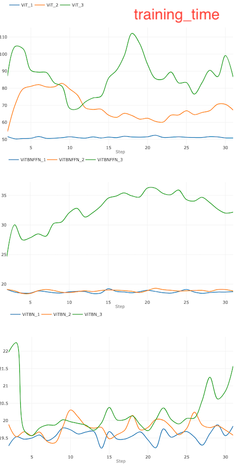
It is evident that the variation of the training time with learning rate is most significant for ViT (top figure). On the other hand, the training time for ViTBN remains roughly the same as we vary the learning rate (bottom figure). For ViTBNFFN, the variation becomes significant only at a relatively large value (~0.01) of the learning rate (middle figure).
Experiment 2: Comparing the Optimized Models
Let us now set up the experiment where we compare the performance of the optimized models. This will involve the following steps:
- First perform a Bayesian optimization to determine the best set of hyperparameters — learning parameter and batch size — for each model.
- Given the three optimized models, train and test each of them for 30 epochs and compare the metrics using MLFlow as before — in particular, the training and testing/inference times per epoch.
Let us begin with the first step. We use the BoTorch optimization engine available on the Ax platform. For details on the optimization procedure using BoTorch, we refer the reader to this documentation on Ax. We use accuracy as the optimization metric and limit the optimization procedure to 20 iterations. We also need to specify the ranges of hyperparameters over which the search will be performed in each case. Our previous experiments give us some insight into what the appropriate ranges should be. The learning parameter range is [1e-5, 1e-3] for ViT, while that for ViTBNFFN and ViTBN is [1e-5, 1e-2]. For all three models, the batch size range is [20, 120]. The complete code for the optimization procedure can be found in the module hypopt_train.py in the optimization folder of the github repo.
The upshot of the procedure is a set of optimized hyperparameters for each model. We summarize them in Table 2.

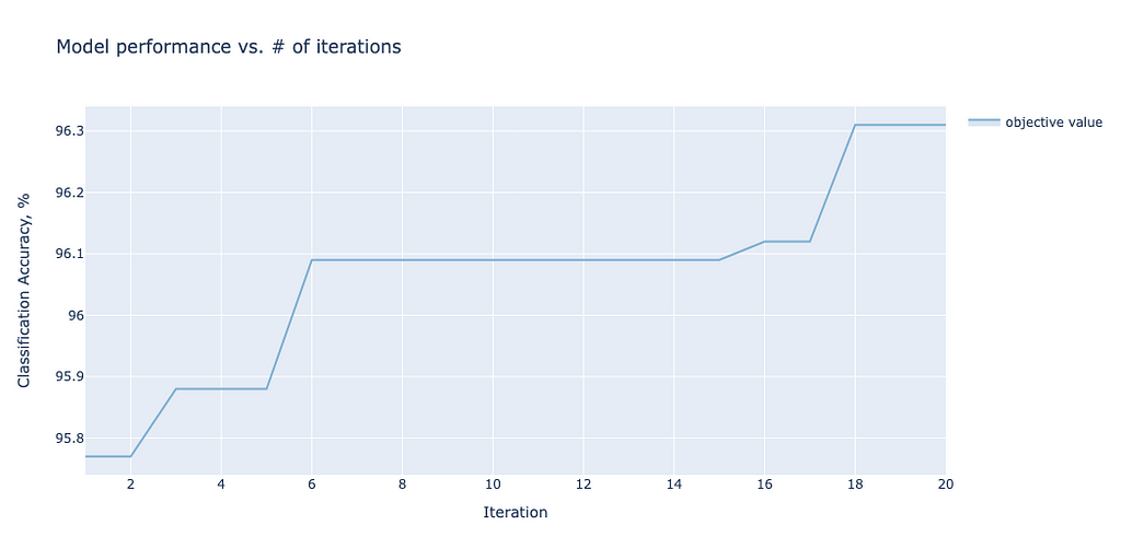
For each model, one can plot how the accuracy converges as a function of the iterations. As an illustrative example, we show the convergence plot for ViTBNFFN in Figure 7.
One can now embark on step 2 — we train and test each model with the optimized hyperparameters for 30 epochs. The comparison of the metrics for the models for 30 epochs of training and testing is summarized in the set of four graphs in Figure 8.
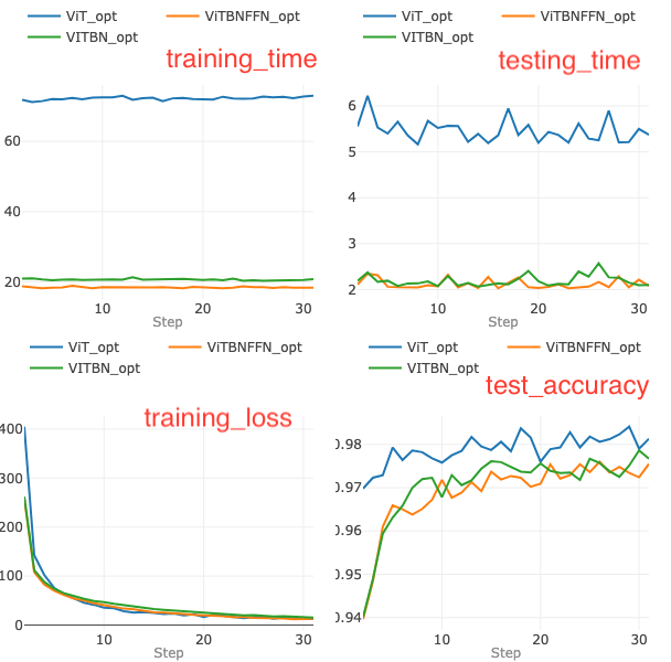
At the end of 30 epochs, the models — ViT, ViTBNFFN and ViTBN — achieve 98.1%, 97.6 % and 97.8% accuracies respectively. ViT converges in a fewer number of epochs compared to ViTBNFFN and ViTBN.
From the two graphs on the top row of Figure 8, one can readily see that the models with BatchNorm are significantly faster in training as well as in inference per epoch. For ViTBNFFN, the ratios rₜ and rᵥ can be computed from the above data : rₜ (ViTBNFFN) = 3.9 and rᵥ(ViTBNFFN)= 2.6, while for ViTBN, we have rₜ (ViTBN) = 3.5 and rᵥ(ViTBN)= 2.5. The resulting gains in average training time per epoch and average inference time per epoch (gₜ and gᵥ respectively) are summarized in Table 3.

A Brief Summary of the Results
Let us now present a quick summary of our investigation :
- Gain in Training and Testing Speed at Fixed Learning Rate: The average training time per epoch speeds up significantly for both ViTBNFFN and ViTBN with respect to ViT. The gain gₜ is >~ 60% throughout the range of learning rates probed here, but may vary significantly depending on the learning rate and the model as evident from Table 1. For the average testing time per epoch, there is also a significant gain (~60%) but this remains roughly the same over the entire range of learning rates for both models.
- Gain in Training and Testing Speed for Optimized Models: The gain in average training time per epoch is above 70% for both ViTBNFFN and ViTBN while the gain in the inference time is a little above 60% — the precise values for gₜ and gᵥ are summarized in Table 3. The optimized ViT model converges faster than the models with BatchNorm.
- BatchNorm and Higher Learning Rate : For smaller learning rate (~ 0.0005), all three models are stable with ViT converging faster compared to ViTBNFFN/ViTBN. For the intermediate learning rate (~ 0.005), the three models have very similar convergences. For higher learning rate (~ 0.01), ViT becomes unstable while the models ViTBNFFN/ViTBN remain stable with an accuracy comparable to the case of the intermediate learning rate. Our findings, therefore, confirm the general expectation that integrating BatchNorm in the architecture allows one to use higher learning rates.
- Variation of Training Time with Learning Rate : For ViT, there is a large increase in the average training time per epoch as one dials up the learning rate, while for ViTBNFFN this increase is much smaller. On the other hand, for ViTBN the training time varies the least. In other words, the training time is most stable with respect to variation in the learning rate for ViTBN.
Concluding Remarks
In this article, I have introduced two models which integrate BatchNorm in a ViT-type architecture — one of them deploys BatchNorm in the feedforward network (ViTBNFFN) while the other replaces LayerNorm with BatchNorm everywhere (ViTBN). There are two main lessons that we learn from the numerical experiments discussed above. Firstly, models with BatchNorm significantly speed up both the training and inference for a ViT. For the MNIST dataset, the training and testing times per epoch speed up by at least 60% in the range of learning rates I consider. Secondly, models with BatchNorm allow one to use a larger learning rate during training without rendering the model unstable.
Also, in this article, I have focused my attention exclusively on the standard ViT architecture. However, one can obviously extend the discussion to other transformer-based architectures for computer vision. The integration of BatchNorm in transformer architecture has been addressed for the DeiT (Data efficient image Transformer) and the Swin Transformer by Yao et al. I refer the reader to this paper for details.
Thanks for reading! If you have made it to the end of the article, please do not forget to leave a comment! Unless otherwise stated, all images and graphs used in this article were generated by the author.
Speeding Up the Vision Transformer with BatchNorm was originally published in Towards Data Science on Medium, where people are continuing the conversation by highlighting and responding to this story.
Originally appeared here:
Speeding Up the Vision Transformer with BatchNorm
Go Here to Read this Fast! Speeding Up the Vision Transformer with BatchNorm
