Text Vectorization Demystified: Transforming Language into Data

An intuitive guide to text vectorization

In my last post, we took a closer look at foundation models and large language models (LLMs). We tried to understand what they are, how they are used and what makes them special. We explored where they work well and where they might fall short. We discussed their applications in different areas like understanding text and generating content. These LLMs have been transformative in the field of Natural Language Processing (NLP).

When we think of an NLP Pipeline, feature engineering (also known as feature extraction or text representation or text vectorization) is a very integral and important step. This step involves techniques to represent text as numbers (feature vectors). We need to perform this step when working on NLP problem as computers cannot understand text, they only understand numbers and it is this numerical representation of text that needs to be fed into the machine learning algorithms for solving various text based use cases such as language translation, sentiment analysis, summarization etc.

For those of us who are aware of the machine learning pipeline in general, we understand that feature engineering is a very crucial step in generating good results from the model. The same concept applies in NLP as well. When we generate numerical representation of textual data, one important objective that we are trying to achieve is that the numerical representation generated should be able to capture the meaning of the underlying text. So today, in our post we will not only discuss the various techniques available for this purpose but also evaluate how close they are to our objective at each step.

Some of the prominent approaches for feature extraction are:

– One hot encoding

– Bag of Words (BOW)

– ngrams

– TF-IDF

– Word Embeddings

We will start by understanding some basic terminologies and how they relate to each other.

– Corpus — All words in the dataset

– Vocabulary — Unique words in the dataset

– Document — Unique records in the dataset

– Word — Each word in a document

E.g. For the sake of simplicity, let’s assume that our dataset has only three sentences, the following table shows the difference between the corpus and vocabulary.

Now each of the three records in the above dataset will be referred to as the document (D) and each word in the document is the word(W).

Let’s now start with the techniques.

1. One Hot Encoding:

This is one of the most basic techniques to convert text to numbers.

We will use the same dataset as above. Our dataset has three documents — we can call them D1, D2 and D3 respectively.

We know the vocabulary (V) is [Cat, plays, dog, boy, ball] which is having 5 elements in it. In One Hot Encoding (OHE), we are representing each of the words in each document based on the vocabulary of the dataset. “1” appears in positions where there is a match.

We can therefore use the above to derive One Hot Encoded representation of each of the documents.

What we are essentially doing here is that we are converting each word of our document into a 2- dimensional vector where the first dimension is the number of words in the document and the second value indicate the vocabulary size (V=5 in our case).

Though it is very easy to understand and implement, there are some drawbacks of this method due which this technique is not preferred to be used.

– Sparse representation (meaning there are lots of 0s and for each word for only one position there is a 1). Bigger the corpus, bigger is the V value and more will be the sparsity.

– Suffers from Out of Vocabulary problems — meaning if there is a new word (a word which is not present in V while training) is introduced at inference time, the algorithm fails to work.

– Last and most important point, this does not capture the semantic relationship between words (which is our primary objective if you remember our discussion above).

That leads us to explore the next technique

2. Bag of Words (BOW)

It is a very popular and quite old technique.

First step is to again create the Vocabulary (V) from the dataset. Then, we compare the number of occurrences of each word from the document against Vocabulary created. The following demonstration using earlier data will help to understand better

In the first document, “cat” appears once, “plays” appears once and so does the “ball”. So, 1 is the count for each of those words and the other positions are marked 0. Similarly, we can arrive at the respective counts for each of the other two documents.

The BOW technique converts each document into a vector of size equal to the Vocabulary V. Here we get three 5 dimensional vectors — [1,1,0,0,1], [0,1,1,0,1] and [0,1,0,1,1]

Bag of Words is used in classification tasks and has been found to perform quite well. And if you look at the table you can understand that it also helps to capture the similarity between the sentences -atleast little . For e g: “plays” and “ball” appears in all the three documents and hence we can see 1 at those positions for all the three documents.

Pros:

– Very easy to understand and implement

– Fixed length problem found earlier does not happen here , as the counts are calculated based on the existing Vocabulary which in turns helps to solve the Out Of Vocabulary problem identified in earlier technique. So, if a new word appears in the data at inference time, the calculations are done based on the existing words and not on new words.

Cons:

– This is still a sparse representation which is difficult for computation

– Though we don’t get error as earlier when a new word comes as only the existing words are considered, we are actually losing information by ignoring the new words.

– It does not consider the sequence of words as order of words can be very important in understanding the text concerned

– When documents have common words most of the time but when a small change can convey opposite meaning, then BOW fails to work. E.g.:

E.g.: Suppose there are two sentences –

1. I like when it rains.

2. I don’t like when it rains.

With the way BOW is calculated, we can see both sentences will be considered similar as all words except “don’t” are present in both sentences, but that single word completely changes the meaning of the second sentence when compared to the first.

3. Bag of Words (BOW) — ngrams

This technique is similar to BOW which we learnt just now but this time, instead of single words, our vocabulary will be made using ngrams ( 2 words together known as bigrams, 3 words together known as trigrams .. or to address it in a generic manner — n words together known as “ngrams”)

Ngrams technique is an improvement on top of Bag of Words as it helps to capture the semantic meaning of the sentences, again at least to some extent. Let’s consider the example used above.

1. I like when it rains.

2. I don’t like when it rains.

These two sentences are completely opposite in meaning and their vector representations should therefore be far off.

When we use only the single words i.e. BOW with n=1 or unigrams, their vector representation will be as follows

D1 can represented as [1,1,1,1,1,0] while D2 can be represented as [1,1,1,1,1,1].

D1 and D2 appear to be very similar and the difference seems to happen in only 1 dimension. Therefore, they can be represented quite close to each other when plotted in a vector space.

Now, let’s see how using bigrams may be more useful in such a situation.

With this approach we can see the values do not match across three dimensions which definitely helps to represent the dissimilarity of the sentences better in the vector space when compared to the earlier technique.

Pros

· It is a very simple & intuitive approach that is easy to understand and implement

· Helps to capture the semantic meaning of the text, at least to some extent

Cons:

· Computationally more expensive as instead of single tokens , we are using a combination of tokens now. Using n-grams significantly increases the size of the feature space. For instance, in practical cases we will not be dealing with few words , rather our vocabulary of can have words in thousands, the number of possible bigrams will be very high.

· This kind of data representation is still sparse. As n-grams capture specific sequences of words, many n-grams might not appear frequently in the corpus, resulting in a sparse matrix.

· The OOV problem still exits. If a new sentence comes in, it will be ignored as similar to BOW technique only the existing words/bigrams present in the vocabulary will be considered.

It is possible to use ngrams(bigrams , trigrams etc) along with unigrams and may help to achieve good results in certain usecases.

For the techniques that we discussed above till now, we have used the value at each position based on the presence or absence or a specific word/ngrams or the frequency of the word/ngrams.

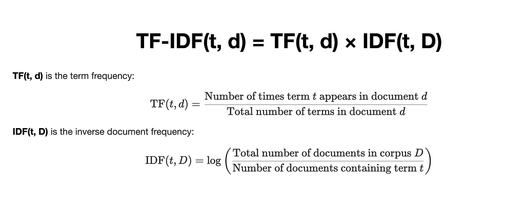
4. Term Frequency — Inverse Document (TF-IDF) Frequency.

This technique employs a unique logic (formula) to calculate the weights for each word based on two aspects –

Term frequency (TF)– indicator of how frequently a word appears in a document. It is the ratio of the number of times a word appears in a document to the total number of words in the document.

Inverse Document Frequency (IDF) on the other hand indicates the importance of a term with respect to the entire corpus.

Formula of TF-IDF:

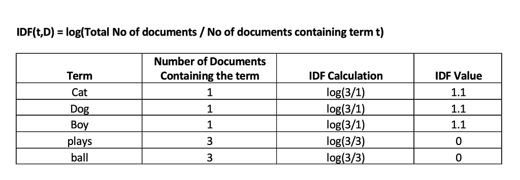
Let’s go through the calculation now using our corpus with three documents.

1. Cat plays ball (D1)

2. Dog plays ball (D2)

3. Boy plays ball (D3)

We can see from the above table that the effect of words occurring in all the documents (plays and ball) has been reduced to 0.

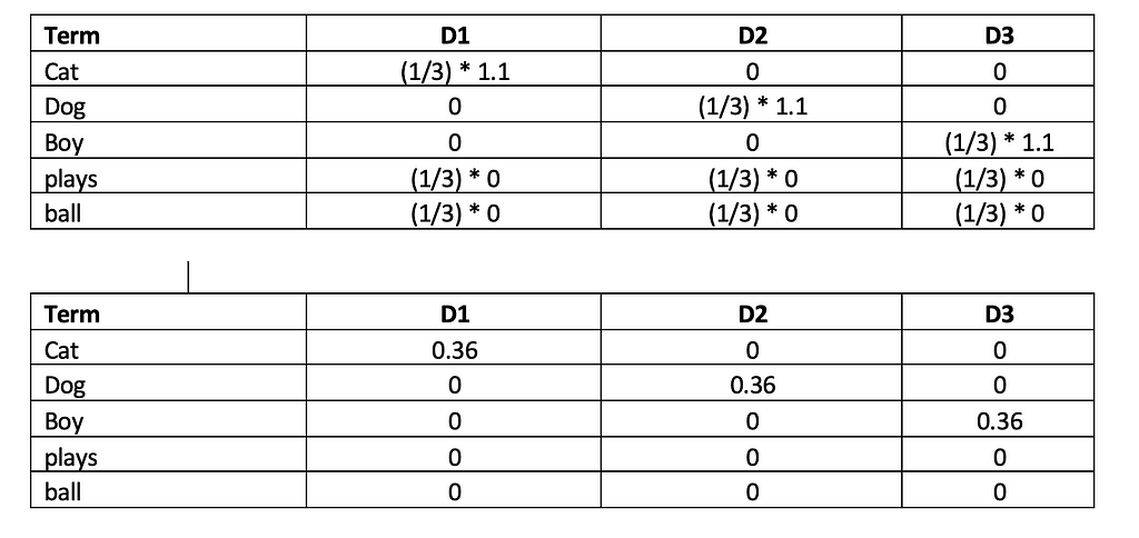
Calculating the TF-IDF using the formula TF-IDF(t,d)=TF(t,d)×IDF(t,D)

We can see how the common words “plays” and “ball” gets dropped and more important words such as “Cat”, “Dog” and “Boy” are identified.

Thus, the approach helps to assigns higher weights to words which appear frequently in a given document but appear fewer times across the whole corpus. TF-IDF is very useful in machine learning tasks such a text classification, information retrieval etc.

We will now move on to learn more advanced vectorization technique.

5. Word Embeddings

I will start this topic by quoting the definition of word embeddings explained beautifully at link

“ Word embeddings are a way of representing words as vectors in a multi-dimensional space, where the distance and direction between vectors reflect the similarity and relationships among the corresponding words.”

Unlike traditional techniques we discussed above ,which are based on word counts or frequencies, word embeddings is a deep learning based technique that can capture the semantic relationships between words. Words that have similar meanings or often appear in similar contexts will have similar vector representations. For example, words like “look” and “see,” which have related meanings, will have similar vectors.

Each word is represented in an n-dimensional space where each dimension captures some aspect of the word’s meaning. These dimensions are not manually defined but are learnt automatically during training. As a neural network is trained on a large corpus of text, it adjusts the word vectors based on the contexts in which words appear, effectively learning their meanings in the process.

There are two primary methods for generating word embeddings:

1. Continuous Bag of Words (CBOW): Predicts a word based on its surrounding context words. This method works well with smaller datasets and shorter context windows.
2. Skip-gram: Predicts the surrounding context words given the current word. It is particularly effective for larger datasets and capturing broader contexts.

To understand better , let us revisit our example sentences:

• Cat plays ball (D1)
• Dog plays ball (D2)
• Boy plays ball (D3)

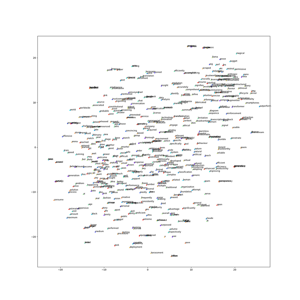
Word embeddings represent each word as a vector in a multi-dimensional space, where the proximity between vectors reflects their semantic similarity.

Considering a simplified 3-D space where the dimensions represent three features — “alive”, “action word” and “intelligence” :

• “Cat” might be represented as [1.0, 0.1, 0.5]
• “Dog” might be represented as [1.0, 0.1, 0.6]
• “Boy” might be represented as [1.0, 0.1, 1.0]
• “plays” might be represented as [0.01, 1.0, 0.002]
• “ball” might be represented as [0.01, 0.4, 0.001]

Here, “Cat” and “Dog” have similar vectors, indicating their semantic similarity, both being animals. “Boy” will have different representation but it is still represents a living being, “plays” and “ball” are also close to each other, which might be because of their frequent occurrence in similar contexts.

Popular Techniques for generating word embeddings

1. Word2Vec: Word2Vec, developed by Google, uses two architectures — Continuous Bag of Words (CBOW) and Skip-gram. It captures the meaning of words in a dense vector space, allowing for tasks like word similarity, analogy completion (e.g., “King” is to “Queen” as “Man” is to “Woman”)

2. GloVe (Global Vectors for Word Representation): Developed by Stanford, GloVe us generates word embeddings by analysing how frequently words co-occur in a large text corpus. This helps GloVe understand both the immediate and overall context of words.

3. FastText: FastText, created by Facebook, improves on the Word2Vec model by looking at parts of words, like chunks of characters. This is helpful because it can understand and process words that are complicated or new, including misspelled words, better than Word2Vec.

Pros

1. Semantic meaning of the language gets captured which could not be achieved earlier

2. Vectors with previous techniques used to be of very high dimensions such are thousands to ten thousands based on the number of words in corpus , which is now reduced to a few hundreds. This helps in faster computation.

3. Dense vector representation of words — mostly non zero values in the vector unlike earlier techniques where we had sparse representation.

Cons

1. It is a deep learning based technique — requires large datasets and lot of computational resources
2. Pre-trained embeddings can struggle with new or rare words.(Out of Vocabular problem)
3. The dimensions of word embeddings are not easily interpretable i.e. we do not get to know what feature or attribute what value at each position in vector represents.

In this blog post, we explored the most popular techniques for converting text into numerical data, which is a key part of Natural Language Processing (NLP). We started with basic methods like One-Hot Encoding and Bag of Words that are very simple to understand but have their own drawbacks, such as creating large, sparse matrices and not capturing the meaning of words well. We then looked at more advanced techniques, like n-grams and TF-IDF which improve on the basic methods by considering word frequency and context, but they still have issues with computational complexity and handling new words. Finally, we discussed word embeddings, a modern approach that leverages deep learning to better understand word relationships.

Each technique has its pros and cons, and the best choice depends on the specific problem we are trying to solve. With the growing interest in NLP and AI, having a clear understanding of these methods will enable us to make informed decisions and achieve better results. The way we represent the data can significantly impact the results. Therefore, choosing the right approach is crucial for success in this evolving and exciting field of NLP & Generative AI.

NOTE : Unless otherwise stated, all images are by the author.

Text Vectorization Demystified: Transforming Language into Data was originally published in Towards Data Science on Medium, where people are continuing the conversation by highlighting and responding to this story.