Event Study Designs: A Very Beginner’s Guide

Event Study Designs: A Beginner’s Guide

What are they and what are they not

In this article, I attempt to clarify the use of essential tools in the applied econometrician’s toolkit: Difference-in-Differences (DiD) and Event Study Designs. Inspired mostly by my students, this article breaks down the basic concepts and addresses common misconceptions that often confuse practitioners.

If you wonder why the title focuses on Event Studies while I am also talking about DiD, it is because, when it comes to causal inference, Event Studies are a generalization of Difference-in-Differences.

But before diving in, let me reassure you that if you are confused, there may be good reasons for it. The DiD literature has been booming with new methodologies in recent years, making it challenging to keep up. The origins of Event Study designs don’t help either…

Origins of Event Studies

Finance Beginnings

Event studies originated in Finance, developed to assess the impact of specific events, such as earnings announcements or mergers, on stock prices. The event study was pioneered by Ball and Brown (1968) and laid the groundwork for the methodology.

Event Studies in Finance

Methodology

In Finance, the event study methodology involves identifying an event window for measuring ‘abnormal returns’, namely the difference between actual and expected returns.

Finance Application

In the context of finance, the methodology typically involves the following steps:

1. Identifying a specific event of interest, such as a company’s earnings announcement or a merger.
2. Determining an “event window,” or the time period surrounding the event during which the stock price might be affected.
3. Calculating the “abnormal return” of the stock by comparing its actual performance during the event window to the performance of a benchmark, such as a market index or industry average.
4. Assessing the statistical significance of the abnormal return to determine whether the event had an impact on the stock price.

This methodological approach has since evolved and expanded into other fields, most notably economics, where it has been adapted to suit a broader range of research questions and contexts.

Evolution into Economics — Causal Inference

Adaptation in Economics

Economists use Event Studies to causally evaluate the impact of economic shocks, and other significant policy changes.

Before explaining how Event Studies are used for causal inference, we need to touch upon Difference-in-Differences.

Differences-in-Differences (DiD) Approach

The DiD approach typically involves i) a policy adoption or an economic shock, ii) two time periods, iii) two groups, and iv) a parallel trends assumption.

Let me clarify each of them here below:

• i) A policy adoption may be: the use of AI in the classroom in some schools; expansion of public kindergartens in some municipalities; internet availability in some areas; cash transfers to households, etc.
• ii) We denote “pre-treatment” or “pre-period” as the period before the policy is implemented and “post-treatment” as the period after the policy implementation.
• iii) We call as “treatment group” the units that are affected by the policy, and “control group” units that are not. Both treatment and control groups are composed of several units of individuals, firms, schools, or municipalities, etc.
• iv) The parallel trends assumption is fundamental for the DiD approach. It assumes that in the absence of treatment, treatment and control groups follow similar trends over time.

A common misconception about the DiD approach is that we need random assignment.

In practice, we don’t. Although random assignment is ideal, the parallel trends assumption is sufficient for estimating causally the effect of the treatment on the outcome of interest.

Randomization, however, ensures that differences between the groups before the intervention are zero, and non-statistically significant. (Although by chance they may be different.)

Scenario: Adoption of ChatGPT in Schools and Emotional Intelligence Performance

Background

Imagine a scenario in which AI becomes available in the year 2023 and some schools immediately adopt AI as a tool in their teaching and learning processes, while other schools do not. The aim is to understand the impact of AI adoption on student emotional intelligence (EI) scores.

Data

• Treatment Group: Schools that adopted AI in 2023.
• Control Group: Schools that did not adopt AI in 2023.
• Pre-Treatment: Academic year before 2023.
• Post-Treatment: Academic year 2023–2024.

Methodology

1. Pre-Treatment Comparison: Measure student scores for both treatment and control schools before AI adoption.
2. Post-Treatment Comparison: Measure student scores for both treatment and control schools after AI adoption.
3. Calculate Differences:

• Difference in test scores for treatment schools between pre-treatment and post-treatment.
• Difference in test scores for control schools between pre-treatment and post-treatment.

The DiD estimate is the difference between the two differences calculated above. It estimates the causal impact of AI adoption on EI scores.

A Graphical Example

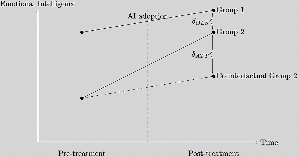
The figure below plots the emotional intelligence scores in the vertical axis, whereas the horizontal axis measures time. Our time is linear and composed of pre- and post-treatment.

The Counterfactual Group 2 measures what would have happened had Group 2 not received treatment. Ideally, we would like to measure Contrafactual Group 2, which are scores for Group 2 in the absence of treatment, and compare it with observed scores for Group 2, or those observed once the group receives treatment. (This is the main issue in causal inference, we can’t observe the same group with and without treatment.)

If we’re tempted to do the naive comparison between the outcomes of Group 1 and Group 2 post-treatment, we would get an estimate that won’t be correct, it will be biased, namely delta OLS in the figure.

The difference-in-differences estimator allows us to estimate the causal effect of AI adoption, shown geometrically in the figure as delta ATT.

The plot indicates that schools where students had lower emotional intelligence scores initially adopted AI. Post-treatment, the scores of the treatment group almost caught up with the control group, where the average EI score was higher in the pre-period. The plot suggests that in the absence of treatment, scores would have increased for both groups — common parallel trends. With treatment, however, the gap in scores between Group 2 and Group 1 is closing.

Note that units in the control group can be treated at another point in time, namely in 2024, 2025, 2026, and so on. What’s important is that in the pre-treatment period, none of the units, in treatment or control groups, is affected by the policy (or receives treatment).

If we only have two time periods, the control group, in our study, will be, by design, a “never treated” group.

DiD for Multiple Periods

When different units receive treatment at different points in time, we can establish a more generalized framework for estimating causal effects. In this case, each group will have a pre-treatment period and a post-treatment period, delineated by the introduction/adoption of the policy (or the assignment to treatment) for each unit.

Back to our Event Study Design

As mentioned, Event Study Designs are a flavor of generalized Difference-in-Differences. Such designs allow researchers to flexibly estimate the effects of the policy or allocation to treatment.

We estimate Event Studies with a linear estimating equation in which we include leads and lags of the treatment variable, denoted with D, and additional covariates x.

A nice feature of these designs is that the coefficient estimates on the leads and lags will give us a sense of the relevant event window helping us to determine whether the impact is temporary or persistent over time.

Moreover, and most importantly perhaps, the coefficient estimates on the leads indicators will inform us if the parallel trends assumption holds.

A Simulation (with Stata Code).

The simulation ensures that we have data on schools since 2021 (pre-treatment). From 2023 onward, some schools, randomly chosen, adopt AI in 2023, some in 2024, and so on until 2027.

Let’s assume that the treatment causes a 5-unit increase in the year of adoption (for the treatment groups only), and the effect lasts only for one period.

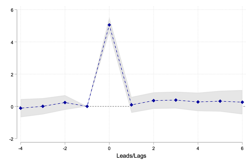
The event study plot will display the coefficient estimates on leads and lags. Our hypothetical scenario will produce a plot similar to the one below.

The coefficient estimates on the lead indicators are close to zero and statistically insignificant, suggesting that the parallel trends assumption holds: treatment and control groups are comparable.

The intervention causes a temporary increase in the outcome of interest by 5 units, after which the treatment effect vanishes.

(Feel free to explore using the code in GitHub ariedamuco/event-study and compare the DiD design with two periods with the event study design, with and without a pure control or a never-treated group.)

GitHub – ariedamuco/event-study

Misconceptions About Event Studies

Misconception 1: Event Studies Are Only for Stock Prices

While commonly associated with stock prices, event studies have broader applications, including analyzing the impact of policy changes, economic events, and more.

Misconception 2: You Always Need a Never-Treated Group

Event Studies, allow us to estimate the effects of the policy without having a “never treated group”.

The staggered treatment in the event study design allows us to create a control group for each treated unit at time t, with the control group being treated at a later time t+n.

In this case, we are closer to comparing apples with apples as we are comparing units that receive treatment with those that will receive treatment in the future.

Misconception 3: You Need an Event Window

The power of event studies lies in their flexibility. Because we can estimate the effect of the treatment over time, the event study allows us to pinpoint the relevant event window.

For example, if there is an anticipatory effect, the event study will show it in the leads, namely the indicator variables leading up to the event will be statistically significant. (Note that this will invalidate the parallel trends assumption.)

Similarly, if the effect is long-lasting, the event study will help capture this feature. In this case, the lags included in the estimating equation will turn out to be significant, and even understand how long the effect persists.

Misconception 4: You Don’t Need Parallel Trend Assumptions

If you don’t have parallel trend assumptions, you are not dealing with a DiD (or Event Studies). However, you can have conditional parallel trend assumptions. This means that the parallel trend assumption holds once we control for covariates. (The covariates should not be affected themselves by the treatment, and ideally, they should be measured pre-treatment.)

Conclusion

Event study designs are a generalization of the Difference-in-Differences approach. Understanding the methodology and addressing common misconceptions ensures that researchers can effectively apply this tool in their empirical research.

Notes

Unless otherwise noted, all images are by the author.

Check out Pedro H. C. Sant’Anna’s and co-authors work on the topic (among others).

Please use this post by Scott Cunningham on the DiD checklist by Pedro H. C. Sant’Anna.

Scott Cunningham’s, Mix Tape, has an excellent introduction to DiD and Event Studies.

A nice introduction on Medium on DiD.

Thank you for taking the time to read about my thoughts. If you enjoyed the article feel free to reach out at [email protected] or on Twitter, Linkedin, or Instagram. Feel free to also share it with others.

About me

Event Study Designs: A Very Beginner’s Guide was originally published in Towards Data Science on Medium, where people are continuing the conversation by highlighting and responding to this story.