Detecting Clouds with AI

From Random Forest to YOLO: Comparing different algorithms for cloud segmentation in satellite Images.

Written by: Carmen Martínez-Barbosa and José Arturo Celis-Gil

Satellite imagery has revolutionized our world. Thanks to it, humanity can track, in real-time, changes in water, air, land, vegetation, and the footprint effects that we are producing around the globe. The applications that offer this kind of information are endless. For instance, they have been used to assess the impact of land use on river water quality. Satellite images have also been used to monitor wildlife and observe the growth of the urban population, among other things.

According to the Union of Concerned Scientists (UCS), approximately one thousand Earth observation satellites are orbiting our planet. However, one of the most known is Sentinel-2. Developed by the European Space Agency (ESA), Sentinel-2 is an earth observation mission from the Copernicus Programme that acquires imagery at high spatial resolution (10 m to 60 m) over land and coastal waters. The data obtained by Sentinel-2 are multi-spectral images with 13 bands that run across the visible, near-infrared, and short-wave infrared parts of the electromagnetic spectrum.

The imagery produced by Sentinel-2 and other Earth observation satellites is essential to developing the applications described above. However, using satellite images might be hampered by the presence of clouds. According to Rutvik Chauhan et al., roughly half of the Earth’s surface is covered in opaque clouds, with an additional 20% being blocked by cirrus or thin clouds. The situation worsens as clouds can cover a region of interest for several months. Therefore, cloud removal is indispensable for preprocessing satellite data.

In this blog, we use and compare different algorithms for segmenting clouds in Sentinel-2 satellite images. We explore various methods, from the classical Random Forest to the state-of-the-art computer vision algorithm YOLO. You can find all the code for this project in this GitHub repository.

Without further ado, let’s get started!

Disclaimer: Sentinel data is free and open to the broad Regional, National, European, and International user community. You can access the data through the Copernicus Open Access Hub, Google Earth Engine, or the Python package sentinelhub. In this blog, we use the last option.

SentinelHub in a nutshell

Sentinelhub is a Python package that supports many utilities for downloading, analyzing, and processing satellite imagery, including Sentinel-2 data. This package offers excellent documentation and examples that facilitate its usage, making it quite prominent when developing end-to-end geo-data science solutions in Python.

To use Sentinelhub, you must create an account in the Sentinel Hub dashboard. Once you log in, go to your dashboard’s “User Settings” tab and create an OAuth client. This client allows you to connect to Sentinehub via API. The steps to get an OAuth client are clearly explained in Sentinelhub’s official documentation.

Once you have your credentials, save them in a secure place. They will not be shown again; you must create new ones if you lose them.

You are now ready to download Sentinel-2 images and cloud probabilities!

Getting the data

In our GitHub repository, you can find the script src/import_image.pythat downloads both Sentinel-2 images and cloud probabilities using your OAuth credentials. We include the file settings/coordinates.yaml that contains a collection of bounding boxes with their respective date and coordinate reference system (CRS). Feel free to use this file to download the data; however, we encourage you to use your own coordinates set.

We download all 13 bands of the images in Digital Numbers (DN). For our purposes, we only use optical (RGB) bands.

Is it necessary to preprocess the data?

The raw images’ DN distribution in the RGB bands is usually skewed, having outliers or noise. Therefore, you must preprocess these data before training any machine learning model.

The steps we follow to preprocess the raw images are the following:

• Usage of a log1p transformation: This helps reduce the skewness of the DN distributions.
• Usage of a min-maxscaling transformation: We do this to normalize the RGB bands.
• Convert DN to pixel values: We multiply the normalized RGB bands by 255 and convert the result to UINT8.

The implementation of these steps can be made in a single function in Python:

The images are cleaned. Now, it’s time to convert the cloud probabilities to masks.

One of the great advantages of using Sentinelhub is that the cloud probabilities come with pixel values on a grayscale. Therefore, every pixel value divided by 255 represents the probability of having a cloud in that pixel. By doing this, we go from values in the range [0, 255] to [0, 1]. Now, to create a mask, we need classes and not probabilities. Thus, we set a threshold of 0.4 to decide whether a pixel has a cloud.

The preprocessing described above enhances the brightness and contrast of the datasets; it is also necessary to get meaningful results when training different models.

Some warnings to consider

In some cases, the resulting mask doesn’t fit the clouds of the corresponding image, as shown in the following picture:

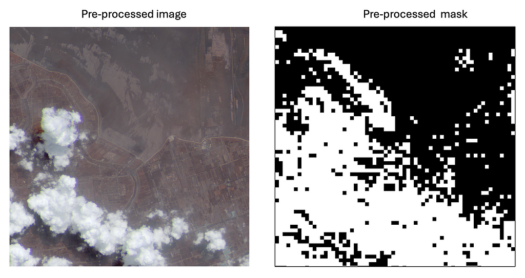
This can be due to multiple reasons: one is the cloud detection model used in Sentinelhub, which returns false positives. Another reason could be the fixed threshold value used during our preprocessing. To resolve this issue, we propose either creating new masks or discarding the image-mask pairs. We chose the second option. In this link, we share a selection of preprocessed images and masks. Feel free to use them in case you want to experiment with the algorithms explained in this blog.

Before modeling, let’s establish a proper metric to evaluate the models’ prediction performance.

Several metrics are used to evaluate an instance segmentation model. One of them is the Intersection over Union (IoU). This metric measures the amount of overlap between two segmentation masks. The IoU can have values from 0 to 1. An IoU=0 means no overlap between the predicted and the real segmentation mask. An IoU=1 indicates a perfect prediction.

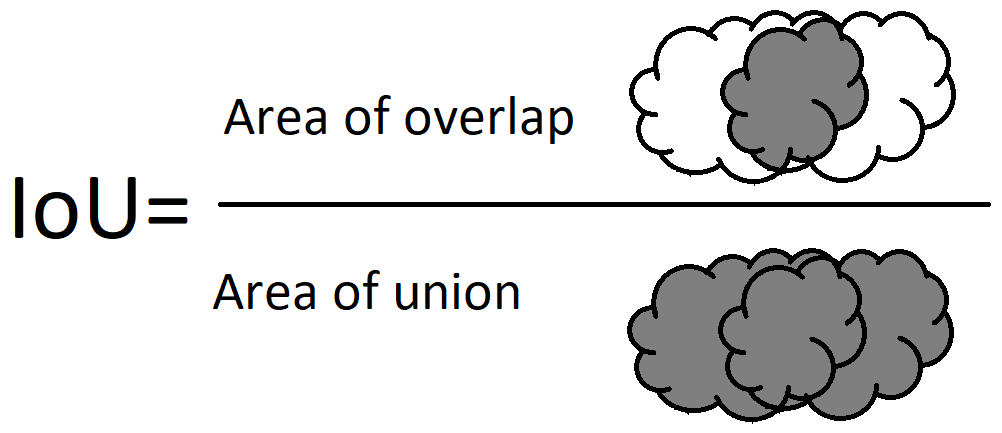
We measure the IoU on one test image to evaluate our models. Our implementation of the IoU is as follows:

Finally, Segmenting clouds in the images

We are now ready to segment the clouds in the preprocessed satellite images. We use several algorithms, including classical methods like Random Forests and ANNs. We also use common object segmentation architectures such as U-NET and SegNet. Finally, we experiment with one of the state-of-the-art computer vision algorithms: YOLO.

Random Forest

We want to explore how well classical methods segment clouds in Satellite images. For this experiment, we use a Random Forest. As known, a Random Forest is a set of decision trees, each trained on a different random subset of the data.

We must convert the images to tabular data to train the Random Forest algorithm. In the following code snippet, we show how to do so:

Note: You can train the models using the preprocessed images and masks by running the script src/model.py in your terminal:

> python src/model.py --model_name={model_name}

Where:

• –model_name=rf trains a Random Forest.
• –model_name=ann trains an ANN.
• –model_name=unet trains a U-NET model.
• –model_name=segnet trains a SegNet model.
• –model_name=yolo trains YOLO.

The prediction over a test image using Random Forest gives the following result:

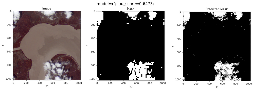
Surprisingly, Random Forest does a good job of segmenting the clouds in this image. However, its prediction is by pixel, meaning this model does not recognize the clouds’ edges during training.

ANN

Artificial Neural Networks are powerful tools that mimic the brain’s structure to learn from data and make predictions. We use a simple architecture with one hidden dense layer. Our aim was not to optimize the ANN’s architecture but to explore the capabilities of dense layers to segment clouds in Satellite images.

As we did for Random Forest, we converted the images to tabular data to train the ANN.

The model predictions on the test image are as follows:

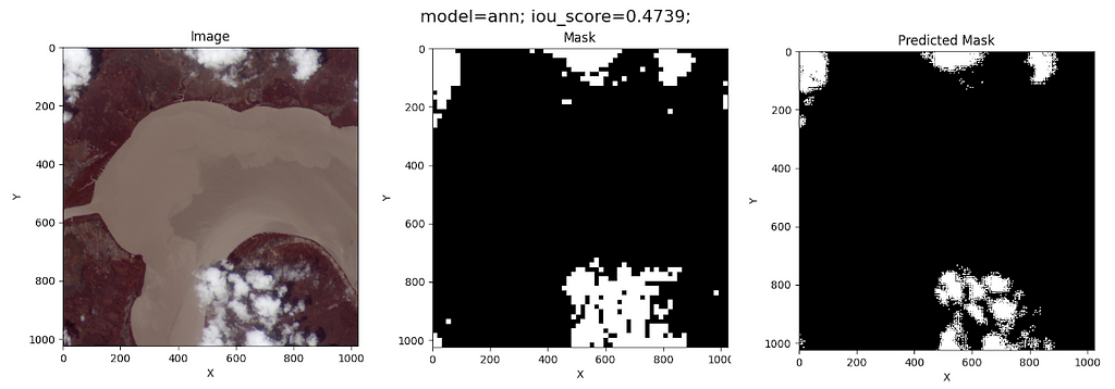
Although this model’s IoU is worse than that of the Random Forest, the ANN does not classify coast pixels as clouds. This fact might be due to the simplicity of its architecture.

U-NET

It’s a convolutional Neural Network developed in 2015 by Olaf Ronneberger et al. (See the original paper here). This architecture is an encoder-decoder-based model. The encoder captures an image’s essential features and patterns, like edges, colors, and textures. The decoder helps to create a detailed map of the different objects or areas in the image. In the U-NET architecture, each convolutional encoder layer is connected to its counterpart in the decoder layers. This is called skip connection.

U-Net is often preferred for tasks requiring high accuracy and detail, such as medical imaging.

Our implementation of the U-NET architecture is in the following code snippet:

The complete implementation of the U-NET model can be found in the script src/model_class.py in our GitHub repository. For training, we use a batch size of 10 and 100 epochs. The results of the U-NET model on the test image are the following:

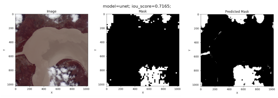
This is the best IoU measurement obtained.

SegNet

It’s another encoder-decoder-based model developed in 2017 by Vijay Badrinarayanan et al. SegNet is more memory-efficient due to its use of max-pooling indices for upsampling. This architecture is suitable for applications where memory efficiency and speed are crucial, like real-time video processing.

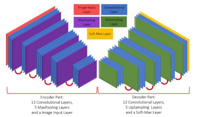
This architecture differs from U-NET in that U-NET uses skip connections to retain fine details, while SegNet does not.

Like the other models, SegNet can be trained by running the script src/model.py. Once more, we use a batch size of 10 and 100 epochs for training. The resulting cloud segmentation on the test image is shown below:

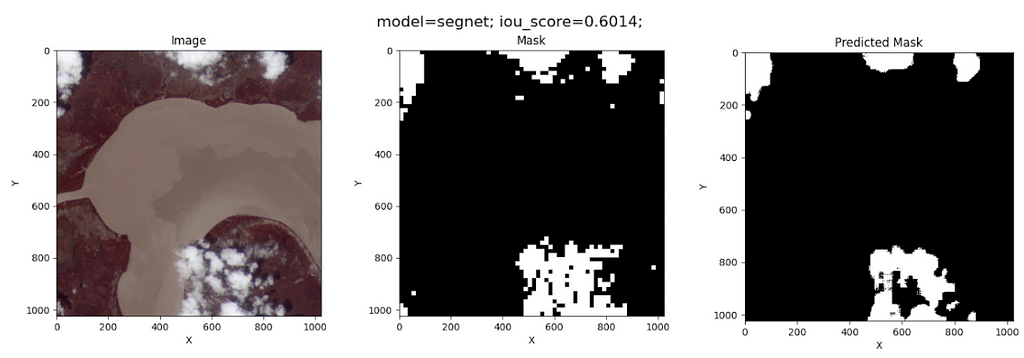
Not as good as U-NET!

YOLO

You Only Look Once (YOLO) is a fast and efficient object detection algorithm developed in 2015 by Joseph Redmon et al. The beauty of this algorithm is that it treats object detection as a regression problem instead of a classification task by spatially separating bounding boxes and associating probabilities to each of the detected images using a single convolutional neural network (CNN).

YOLO’s advantage is that it supports multiple computer vision tasks, including image segmentation. We use a YOLO segmentation model through the Ultralytics Framework. The training is quite simple, as shown in the snippet below:

You just need to set up a dataset.yaml file which contains the paths of the images and labels. More information on how to run a YOLO model for segmentation is found here.

Note: Cloud contours are needed instead of masks to train the YOLO model for segmentation. You can find the labels in this data link.

The results of the cloud segmentation on the test image are the following:

Ugh, this is an ugly result!

While YOLO is a powerful tool for many segmentation tasks, it may perform poorly on images with significant blurring because blurring reduces the contrast between the object and the background. Additionally, YOLO can have difficulty segmenting each object in pictures with many overlapping objects. Since clouds can be blurred objects without well-defined edges and often overlap with others, YOLO is not an appropriate model for segmenting clouds in Satellite images.

We shared the trained models explained above in this link. We did not include Random Forest due to the file size (it’s 6 GB!).

Take away messages

We explore how to segment clouds in Sentinel-2 satellite images using different ML methods. Here are some learnings from this experiment:

• The data obtained using the Python package sentinelhub is not ready for model training. You must preprocess and perhaps adapt these data to a proper format depending on the selected model (for instance, convert the images to tabular data when training Random Forest or ANNs).
• The best model is U-NET, followed by Random Forest and SegNet. It’s not surprising that U-NET and SegNet are on this list. Both architectures were developed for segmentation tasks. However, Random Forest performs surprisingly well. This shows how ML methods can also work in image segmentation.
• The worst models were ANN and YOLO. Due to its simplicity of architecture, we expected ANN not to give good results. Regarding YOLO, segmenting clouds in images is not a suitable task for this algorithm despite being the state-of-the-art method in computer vision. This experiment overall shows that we, as data scientists, must always look for the algorithm that best fits our data.

We hope you enjoyed this post. Once more, thanks for reading!

You can contact us via LinkedIn at:

https://www.linkedin.com/in/jose-celis-gil/

https://www.linkedin.com/in/camartinezbarbosa/

Detecting Clouds with AI was originally published in Towards Data Science on Medium, where people are continuing the conversation by highlighting and responding to this story.