Estimate the unobserved — Moving-Average Model Estimation with Maximum Likelihood in Python

Estimate the Unobserved: Moving-Average Model Estimation with Maximum Likelihood in Python

How unobserved covariates’ coefficients can be estimated with MLE

For those experienced with time series data and forecasting, terms like regressions, AR, MA, and ARMA should be familiar. Linear Regression is a straightforward model with a closed-form parametric solution obtained through OLS. AR models can also be estimated using OLS. However, things become more complex with MA models, which form the second component of the more advanced ARMA and ARIMA models.

The plan for this story:

1. Introducing Moving Average models
2. Discussing why there’s no closed solution for MA model
3. Introducing Maximum Likelihood Estimation method
4. MA(1) ML estimation — Theory and Python code

Moving Average Model

MA models can be described by the following formula:

Here, the thetas represent the model parameters, while the epsilons are the error terms, assumed to be mutually independent and normally distributed with constant variance. The intuition behind this formula is that our time series, X, can always be described by the last q shocks that occurred in the series. It is evident from the formula that each shock impacts only the subsequent q values of X, in contrast to AR models where the effect of a shock persists indefinitely, although gradually diminishing over time.

Closed estimation of a simple model — Linear Regression

As a reminder, the general form of a linear regression equation looks like this:

For forecasting tasks, we typically aim to estimate all the model’s parameters (the betas) using a sample set of x’s and y’s. Given a few assumptions about our model, the Gauss–Markov theorem states that the ordinary least squares (OLS) estimators for the betas have the lowest sampling variance among the class of linear unbiased estimators. In simpler terms, OLS provides us with the best possible estimation of the betas.

So, what is OLS? It is a closed-form solution to a loss function minimization problem:

where the loss function, S, is defined as follows –

In this context, y and X are our sample data and are observable vectors of numbers (as in time series). Therefore, it is straightforward to calculate the function S, determine its derivative, and find the beta that solves the minimization problem.

Closed estimation of MA(q)

It is should be clear why applying a method like OLS to estimate MA(q) models is problematic — the dependent variable, the time series values, are described by unobservable variables, the epsilons. This raises the question: how can these models be estimated at all?

Maximum Likelihood (MLE)

Likelihood Function

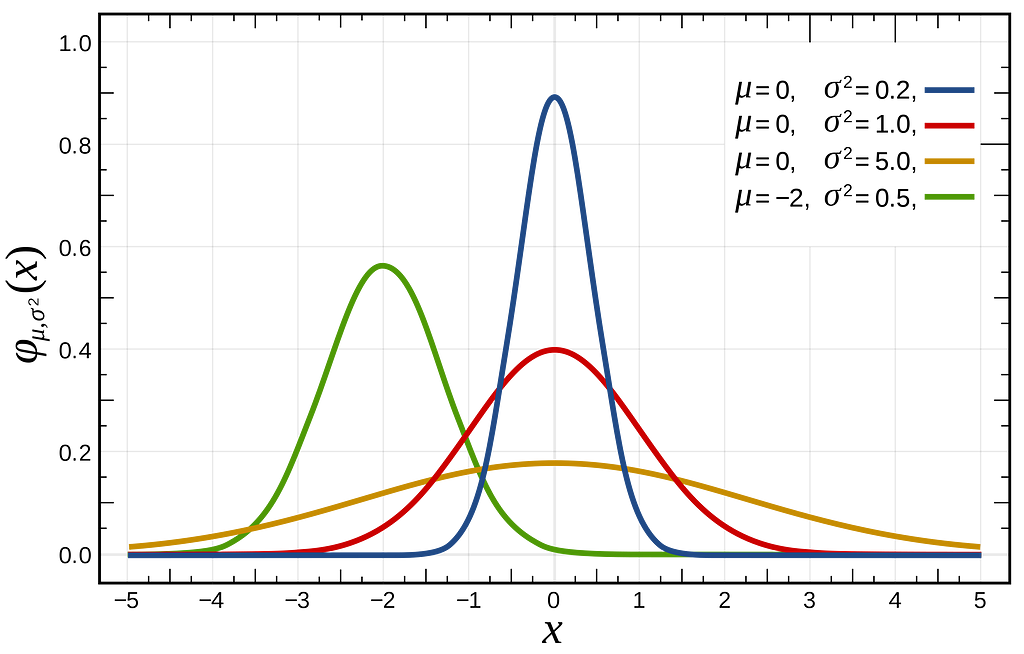
Statistical distributions typically depend on one or more parameters. For instance, the normal distribution is characterized by its mean and variance, which define its “height” and “center of mass” —

Suppose we have a dataset, X={x_1,…x_n}, comprising samples drawn from an unknown normal distribution, with its parameters unknown. Our objective is to determine the mean and variance values that would characterize the specific normal distribution from which our dataset X is most likely to have been sampled.

MLE provides a framework that precisely tackles this question. It introduces a likelihood function, which is a function that yields another function. This likelihood function takes a vector of parameters, often denoted as theta, and produces a probability density function (PDF) that depends on theta.

The probability density function (PDF) of a distribution is a function that takes a value, x, and returns its probability within the distribution. Therefore, likelihood functions are typically expressed as follows:

The value of this function indicates the likelihood of observing x from the distribution defined by the PDF with theta as its parameters.

The goal

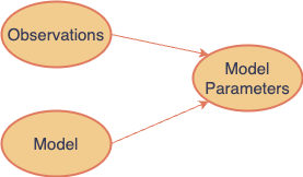
When constructing a forecast model, we have data samples and a parameterized model, and our goal is to estimate the model’s parameters. In our examples, such as Regression and MA models, these parameters are the coefficients in the respective model formulas.

The equivalent in MLE is that we have observations and a PDF for a distribution defined over a set of parameters, theta, which are unknown and not directly observable. Our goal is to estimate theta.

The MLE approach involves finding the set of parameters, theta, that maximizes the likelihood function given the observable data, x.

We assume our samples, x, are drawn from a distribution with a known PDF that depends on a set of parameters, theta. This implies that the likelihood (probability) of observing x under this PDF is essentially 1. Therefore, identifying the theta values that make our likelihood function value close to 1 on our samples, should reveal the true parameter values.

Conditional likelihood

Notice that we haven’t made any assumptions about the distribution (PDF) on which the likelihood function is based. Now, let’s assume our observation X is a vector (x_1, x_2, …, x_n). We’ll consider a probability function that represents the probability of observing x_n conditional on that we have already observed (x_1, x_2, …, x_{n-1}) —

This represents the likelihood of observing just x_n given the previous values (and theta, the set of parameters). Now, we define the conditional likelihood function as follows:

Later, we will see why it is useful to employ the conditional likelihood function rather than the exact likelihood function.

Log-Likelihood

In practice, it is often convenient to use the natural logarithm of the likelihood function, referred to as the log-likelihood function:

This is more convenient because we often work with a likelihood function that is a joint probability function of independent variables, which translates to the product of each variable’s probability. Taking the logarithm converts this product into a sum.

Estimating MA(1) with MLE

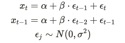
For simplicity, I’ll demonstrate how to estimate the most basic moving average model — MA(1):

Here, x_t represents the time-series observations, alpha and beta are the model parameters to be estimated, and the epsilons are random noise drawn from a normal distribution with zero mean and some variance — sigma, which will also be estimated. Therefore, our “theta” is (alpha, beta, sigma), which we aim to estimate.

Let’s define our parameters and generate some synthetic data using Python:

import pandas as pd
import numpy as np

STD = 3.3
MEAN = 0
ALPHA = 18
BETA = 0.7
N = 1000

df = pd.DataFrame({"et": np.random.normal(loc=MEAN, scale=STD, size=N)})
df["et-1"] = df["et"].shift(1, fill_value=0)
df["xt"] = ALPHA + (BETA*df["et-1"]) + df["et"]

Note that we have set the standard deviation of the error distribution to 3.3, with alpha at 18 and beta at 0.7. The data looks like this —

Likelihood function for MA(1)

Our objective is to construct a likelihood function that addresses the question: how likely is it to observe our time series X=(x_1, …, x_n) assuming they are generated by the MA(1) process described earlier?

The challenge in computing this probability lies in the mutual dependence among our samples — as evident from the fact that both x_t and x_{t-1} depend on e_{t-1) — making it non-trivial to determine the joint probability of observing all samples (referred to as the exact likelihood).

Therefore, as discussed previously, instead of computing the exact likelihood, we’ll work with a conditional likelihood. Let’s begin with the likelihood of observing a single sample given all previous samples:

This is much simpler to calculate because —

All that remains is to calculate the conditional likelihood of observing all samples:

applying a natural logarithm gives:

which is the function we should maximize.

Code

We’ll utilize the GenericLikelihoodModel class from statsmodels for our MLE estimation implementation. As outlined in the tutorial on statsmodels’ website, we simply need to subclass this class and include our likelihood function calculation:

from scipy import stats
from statsmodels.base.model import GenericLikelihoodModel
import statsmodels.api as sm

class MovingAverageMLE(GenericLikelihoodModel):
    def initialize(self):
        super().initialize()
        extra_params_names = ['beta', 'std']
        self._set_extra_params_names(extra_params_names)

        self.start_params = np.array([0.1, 0.1, 0.1])

    def calc_conditional_et(self, intercept, beta):
        df = pd.DataFrame({"xt": self.endog})
        ets = [0.0]
        for i in range(1, len(df)):
            ets.append(df.iloc[i]["xt"] - intercept - (beta*ets[i-1]))

        return ets

    def loglike(self, params):
        ets = self.calc_conditional_et(params[0], params[1])
        return stats.norm.logpdf(
            ets,
            scale=params[2],
        ).sum()

The function loglike is essential to implement. Given the iterated parameter values paramsand the dependent variables (in this case, the time series samples), which are stored as class members self.endog, it calculates the conditional log-likelihood value, as we discussed earlier.

Now let’s create the model and fit on our simulated data:

df = sm.add_constant(df) # add intercept for estimation (alpha)
model = MovingAverageMLE(df["xt"], df["const"])
r = model.fit()
r.summary()

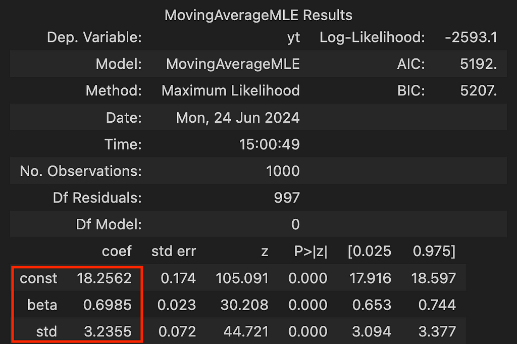
and the output is:

And that’s it! As demonstrated, MLE successfully estimated the parameters we selected for simulation.

Wrapping Up

Estimating even a simple MA(1) model with maximum likelihood demonstrates the power of this method, which not only allows us to make efficient use of our data but also provides a solid statistical foundation for understanding and interpreting the dynamics of time series data.

Hope you liked it !

References

[1] Andrew Lesniewski, Time Series Analysis, 2019, Baruch College, New York

[2] Eric Zivot, Estimation of ARMA Models, 2005

Unless otherwise noted, all images are by the author

Estimate the unobserved — Moving-Average Model Estimation with Maximum Likelihood in Python was originally published in Towards Data Science on Medium, where people are continuing the conversation by highlighting and responding to this story.