Managing Pivot Table and Excel Charts with VBA

Save precious hours by automating working with pivot tables and charts using VBA

As digitalization and innovation are taking over different domains, working with big datasets has become a norm and commonplace in Universities, research organizations, and industries. Automating the common tasks can save several hours for analysts, so they can spend less time on processing and managing data, and more time on the juicy part, which is analyzing and generating insights.

A pivot table is one such tool, which allows generaling several insights from stacked datasets. One can perform tons of analysis just by playing with the field settings of the pivot table based on the requirements. If someone has numerous stacked datasets that can be transformed into pivot tables, how can the pivot tables be refreshed automatically? How can one automate the selection of chart colors based on the series name and manage other chart elements? This blog post gives the answers to such questions by an illustrative example, step by step.

While it could take considerable effort to set up the code in the beginning, once it is set up, it can be very handy and time-saving to analysts who work with numerous large datasets daily. Let’s get started.

Data

I took the sample data from the website of Excel-Easy. This is a nice website containing beginner-friendly tutorials on basic Excel and VBA functionalities. The dataset contains records of fruit and vegetable sales in specific countries in 2016 and 2017. The dataset contains six fields: Order ID, Product, Category, Amount, Date, and Country. I divided this dataset into 2 csv files called results1.csv and results2.csv for creating pivot tables.

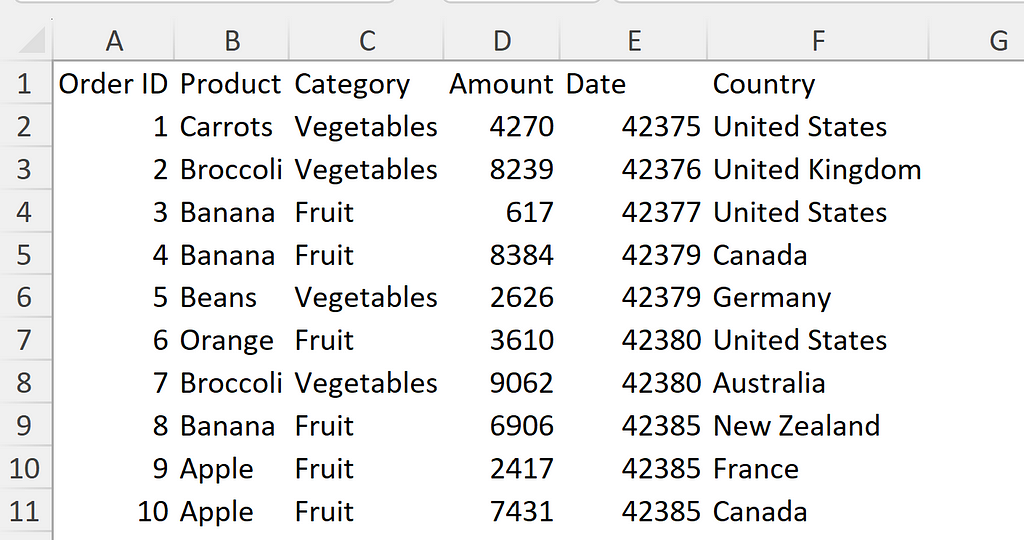
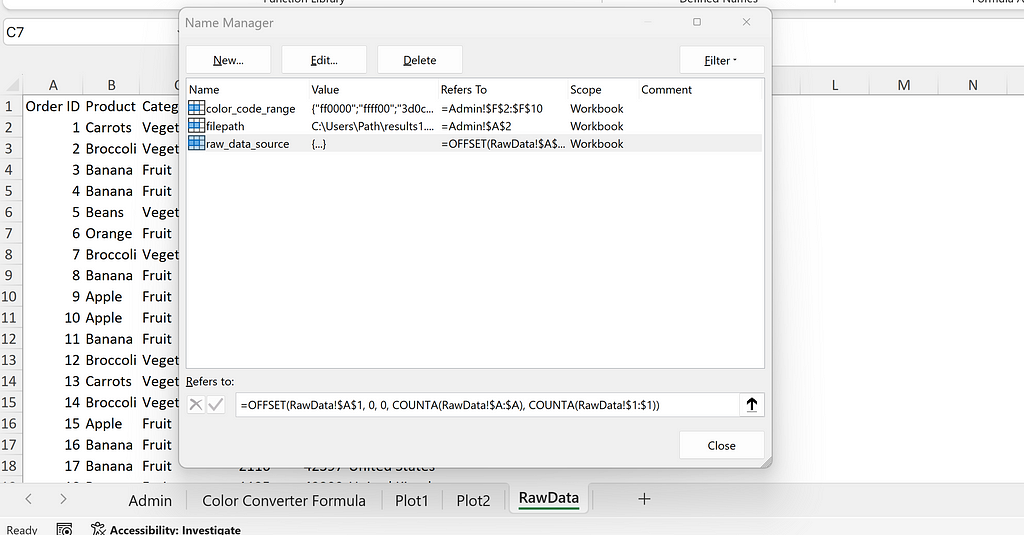
I pulled this dataset in the RawData worksheet. I created a dynamic range called raw_data_source with the following formula:

=OFFSET(RawData!$A$1, 0, 0, COUNTA(RawData!$A:$A), COUNTA(RawData!$1:$1))

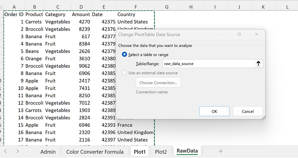
The reason for creating a dynamic range was that the size (number of rows) of the dataset was different in different CSV files, and I wanted to use the entire dataset as source of the pivot table.

Pivot tables and charts

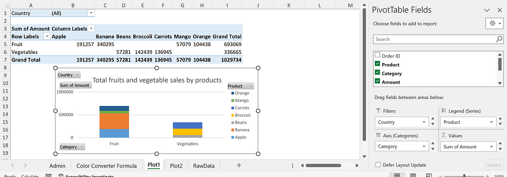
The dataset in the raw_data_source range in the RawData sheet was used as a data source to create two simple pivot tables and charts.

The first one portrayed total fruits and vegetable sales by individual products filterable by country with the field settings as shown.

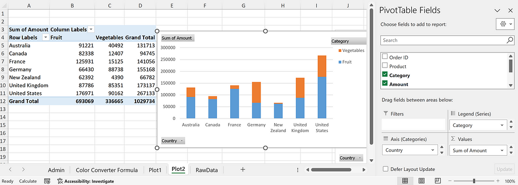
The second one portrayed total fruit and vegetable sales by countries.

1. Automating refreshing pivot tables based on a new dataset

In this step, I wanted to automate the refreshing of the datasets from the file I specified. I created a placeholder in the Admin sheet to place the path of the CSV data whose dataset I wanted to pull and refresh the pivot tables with. I named the cell A2 as filepath as shown below:

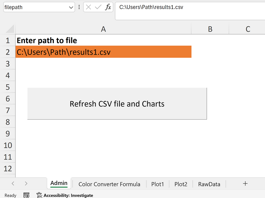
The code for this step is given below in the UpdateRawData subroutine. I declared the variables wb, ws_admin, ws_rawdata, and filepath for the names of the workbook, Admin sheet, RawData sheet, and path of the file containing the dataset respectively. First I cleared the contents of the RawData sheet. Then I went to the source workbook based on the filename, selected the corresponding sheet, copied its contents, returned to the ws_rawdata sheet, and pasted the contents as values. Finally, I refreshed the workbook using the code wb.RefreshAll that refreshed the entire workbook including the sheets with the pivot table and chart respectively.

Sub UpdateRawData()

Dim wb As Workbook
Dim ws_admin As Worksheet
Dim ws_rawdata As Worksheet
Dim filepath As String

Set wb = ThisWorkbook
Set ws_admin = wb.Worksheets(“Admin”)
Set ws_rawdata = wb.Worksheets(“RawData”)

'Clear Rawdata sheet
ws_rawdata.Activate
Cells.Clear

'get file path
filepath = ws_admin.Range(“filepath”)

Application.DisplayAlerts = False

'Open source file and select all contents
Dim src_wb As Workbook
Dim src_ws As Worksheet

Set src_wb = Workbooks.Open(filepath)
Set src_ws = src_wb.Sheets(1)
src_ws.UsedRange.Select

'Copy all
Selection.Copy

'Paste all
ws_rawdata.Range(“A1”).PasteSpecial xlPasteValues

'Close source file
src_wb.Close SaveChanges:=False

wb.RefreshAll

Application.DisplayAlerts = True

End Sub

I linked this subroutine to the Refresh files and charts button. Once I specified the filename in the placeholder and clicked on the button, the dataset and pivot tables were updated automatically.

2. Creating a colors table using VBA

I created a table in the Admin sheet containing the list of the specific fruits and vegetables available in the dataset. In column F, I specified the tentative hexadecimal color codes for the color of each fruit or vegetable. I wanted to use these colors to update the colors in pivot charts. First, I wanted to paint column F with the color I specified in each cell.

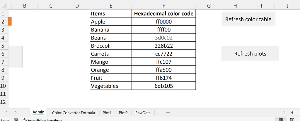
Hexadecimal color code

The hexadecimal code for each color is a 6-digit hexadecimal number (0 to 9 or A to F) with base 16. In a hexadecimal color code RRGGBB, each pair of two letters represents the various shades of red, green, and blue color. In a Red Green Blue (RGB) system, the value of each shade ranges from 0 to 255.

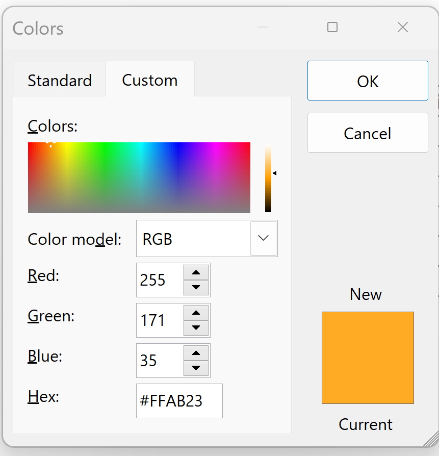
For example, for a hexadecimal color code ffab23, I calculated the corresponding RGB code with the following calculation. ffab23 in the hexadecimal system translates to (255, 171, 35) in the RGB system referring to the Red, Green, and Blue color components respectively.

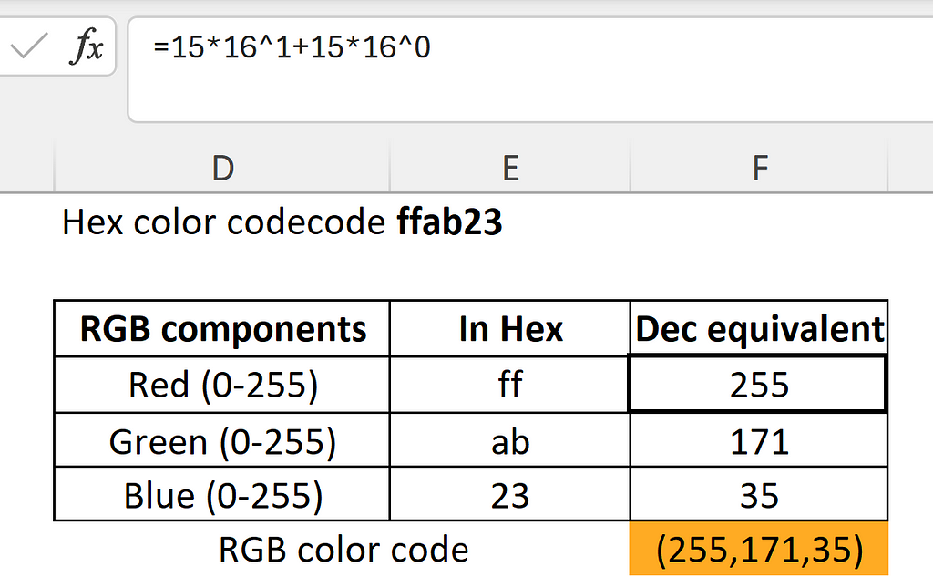
This can also be visualized by going to the Custom Colors option in Excel as shown below:

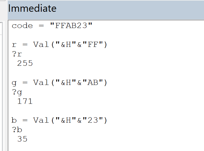
In Excel VBA, using &H in combination with a value implies that it is a hexadecimal number and the Val() function returns the corresponding decimal number. In the Immediate Window below, r, g, and b represent the corresponding decimal values for each shade of Red, Green, and Blue respectively.

In the code below, I created a named range color_code_range for the table containing the hexadecimal color code for each fruit or vegetable. I looped through each cell in the selection, derived the red, green, and blue components in decimal numbers, and painted the interior of the cell with the same RGB color code.

Sub refresh_color_table()

Dim wb As Workbook
Dim ws_admin As Worksheet

Set wb = ThisWorkbook
Set ws_admin = wb.Sheets(“Admin”)
ws_admin.Range("color_code_range").Select
 
Dim c As Range
Dim r, g, b As Long
Dim Hex As String

For Each c In Selection

     Hex = c.Value
 
     r = Val("&H" & Mid(Hex, 1, 2))
     g = Val("&H" & Mid(Hex, 3, 2))
     b = Val("&H" & Mid(Hex, 5, 2))
     c.Interior.Color = RGB(r, g, b)

Next c

End Sub

When I ran the above subroutine, the column F gets painted with the same color as the color code as shown:

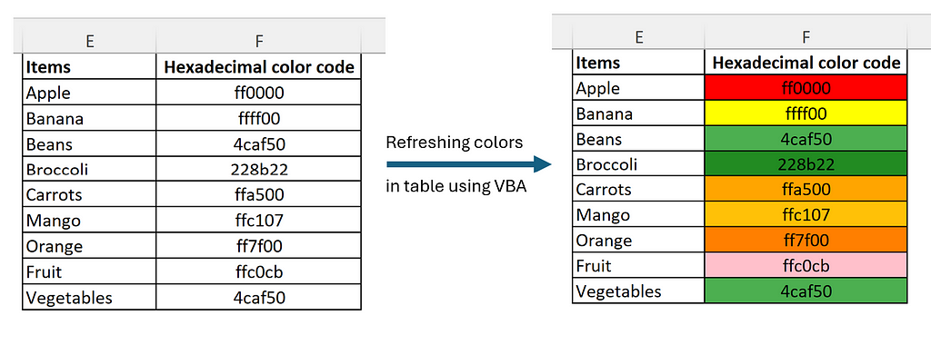
If the color code is changed, and the code is run again, it will generate new colors in the table. Isn’t that cool?

3. Working with a dictionary in VBA

In the next step, I wanted to assign the colors in the pivot charts based on the custom colors I chose above. For this purpose, I created a dictionary containing the product name as keys and the corresponding hexadecimal color codes as values.

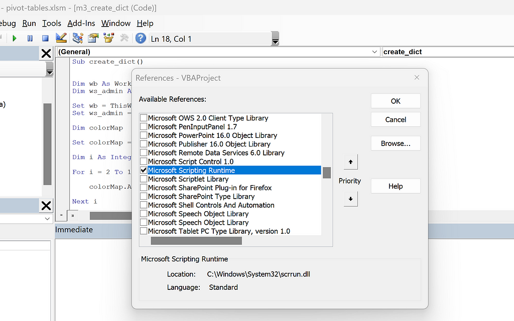
The pre-requisite for creating a dictionary object in VBA is to activate the Microsoft Scripting Runtime beforehand. For this, you can go to Tools -> References -> Check the box next to Microsoft Scripting Runtime and click on ok.

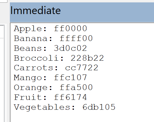
In the code below, I created a dictionary object called colorMap. I looped through the Range E2:F10 in the Admin sheet. I added the contents in column E as keys, and the contents in column F as their corresponding values.

Sub create_dict()

Dim wb As Workbook
Dim ws_admin As Worksheet

Set wb = ThisWorkbook
Set ws_admin = wb.Sheets(“Admin”)

Dim colorMap As Dictionary
Set colorMap = New Dictionary

Dim i As Integer

For i = 2 To 10
    If Not colorMap.Exists(Range("E" & i).Value) Then
        colorMap.Add Range("E" & i).Value, Range("F" & i).Value
    End If
Next i

For Each Key In colorMap.Keys()
     Debug.Print Key & ": " & colorMap(Key)
Next Key

End Sub

In the second for loop above, I looped through each key of the colorMap dictionary and printed the keys and values in the immediate window as shown below:

4. Managing pivot chart elements using VBA

Based on the learnings from the previous steps, I wanted to go one step further and update the pivot chart elements using VBA. In this case, I wanted to set the chart title automatically based on a cell value and apply the colors of specific fruits and vegetables defined in the Admin sheet to the pivot charts.

In this step, I assigned Plot1 and Plot2 sheets as an array called sheetNames. I declared chartObj as ChartObject. Within each sheet, I looped through each ChartObject among all ChartObjects.

Note: ChartObject acts as a container for a Chart object in VBA that controls the size and appearance of the embedded chart in a worksheet. It is a member of the ChartObjects collection. It is important to understand the differences in the methods and properties of each of these objects in VBA.

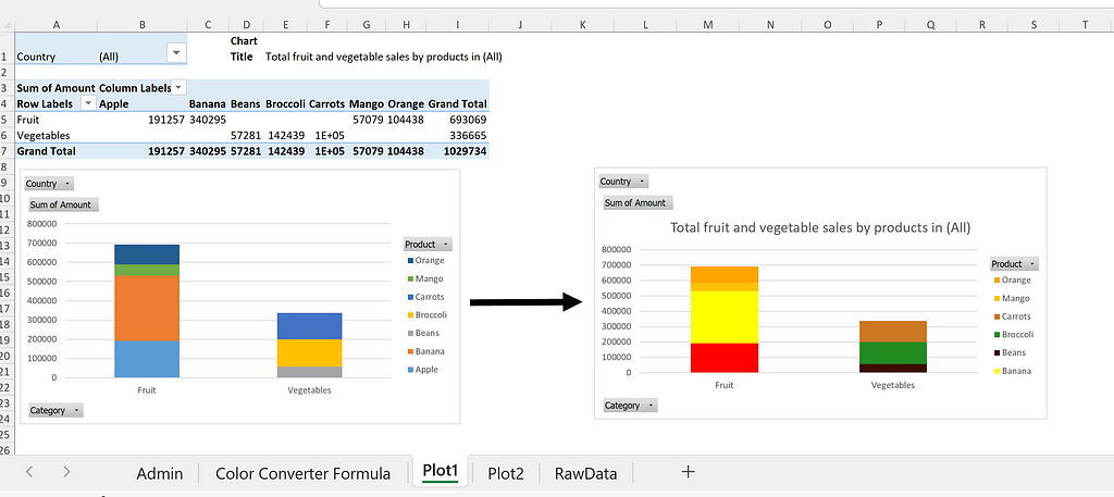
After going through each chartObj, I set the title for each chart based on the value in cell E1. Next, I looped through each series in the overall Series Collection of the Chart object. I assigned the series name (i.e., name of fruit or vegetable) to a variable called itemName, and got the corresponding color code from the colorMap dictionary. Similar to step 2, I got the red, green, and blue components of the color code in decimal numbers, and filled the series bar with the RGB colors.

Sub refresh_plots()

Dim wb As Workbook
Dim ws_admin As Worksheet
Dim ws As Worksheet

Set wb = ThisWorkbook
Set ws_admin = wb.Sheets("Admin")

Dim colorMap
Set colorMap = CreateObject("Scripting.Dictionary")
Dim i As Integer

For i = 2 To 10
     If Not colorMap.Exists(Range("E" & i).Value) Then
          colorMap.Add Range("E" & i).Value, Range("F" & i).Value
     End If
Next i

Dim sheetNames As Variant
Dim sheetName As Variant
sheetNames = Array("Plot1", "Plot2")

Dim hex_color_code As String
Dim r, g, b As Integer

Dim chartObj As ChartObject

For Each sheetName In sheetNames
     Set ws = wb.Sheets(sheetName)
 
     For Each chartObj In ws.ChartObjects
 
          chartObj.Chart.HasTitle = True
          chartObj.Chart.ChartTitle.Text = ws.Range("E1").Value
 
          For Each Series In chartObj.Chart.SeriesCollection

               itemName = Series.Name
               hex_color_code = colorMap(itemName)
 
               r = Val("&H" & Mid(hex_color_code, 1, 2))
               g = Val("&H" & Mid(hex_color_code, 3, 2))
               b = Val("&H" & Mid(hex_color_code, 5, 2))
               Series.Format.Fill.ForeColor.RGB = RGB(r, g, b)
 
          Next Series
     Next chartObj
Next sheetName

End Sub

An illustration of the use of this code is depicted below.

Conclusion

In this post, I illustrated how one can customize and automate working with pivot tables and charts using VBA. I have demonstrated the automation of four key tasks: refreshing pivot tables and charts with new datasets; creating color tables based on hexadecimal color code; how to work with dictionaries in VBA; and managing and updating pivot chart elements using VBA. In the second step, I have elaborated the conversion of hexadecimal color codes to the corresponding RGB color codes using both Excel and VBA, and used this technique in the subsequent steps.

The code and Excel file for this post are present in this GitHub repository. Thank you for reading!

Managing Pivot Table and Excel Charts with VBA was originally published in Towards Data Science on Medium, where people are continuing the conversation by highlighting and responding to this story.