Linear Attention Is All You Need

Self-attention at a fraction of the cost?

“Attention scales badly with long sequence lengths”

This is the kind of thing anyone who’s spent much time working with transformers and self-attention will have heard a hundred times. It’s both absolutely true, we’ve all experienced this as you try to increase the context size of your model everything suddenly comes to a grinding halt. But then at the same time, virtually every week it seems, there’s a new state of the art model with a new record breaking context length. (Gemini has context length of 2M tokens!)

There are lots of sophisticated methods like RingAttention that make training incredibly long context lengths in large distributed systems possible, but what I’m interested in today is a simpler question.

How far can we get with linear attention alone?

Let’s break down the maths.

This will be a bit of a whistle stop tour, but bear with me as we touch on a few key points before digging into the results.

We can basically summarise the traditional attention mechanism with two key points:

• First, the typical softmax attention expression takes the product of the query and key matrices, normalises for stability, then takes the softmax (row wise) to get the attention scores between each element of the sequence.
• Second, the time complexity is dominated by the N² dot products, and the one inside the softmax is the limiting factor. That’s where we compute the attention scores.

This is expressed in the traditional form as:

It turns out if we ask our mathematician friends we can think about this slightly differently. The softmax can be thought of as one of many ways of describing the probability distribution relating tokens with each other. We can use any similarity measure we like (the dot product being one of the simplest) and so long as we normalise it, we’re fine.

It’s a little sloppy to say this is attention, as in fact it’s only the attention we know and love when the similarity function is the exponential of the dot product of queries and keys (given below) as we find in the softmax. But this is where it gets interesting, if instead of using this this expression what if we could approximate it?

We can assume there is some feature map “phi” which gives us a result nearly the same as taking the exponential of the dot product. And crucially, writing the expression like this allows us to play with the order of matrix multiplication operations.

In the paper they propose the Exponential Lineaer Unit (ELU) as the feature map due to a number of useful properties:

1. For values above 0 the ELU(x) gives a linear result, which while not the same as the exponential does preserve the relative ordering between scores.
2. For values less than or equal to 0 the exponential term preserves the continuous nature of the function, and ensures the gradients don’t just vanish.

We won’t spend too much more time on this here, but this is pretty well empirically verified as a fair approximation to the softmax function.

What this allows us to do is change the order of operations. We can take the product of our feature map of K with V first to make a KV block, then the product with Q. The square product becomes over the model dimension size rather than sequence length.

Putting this all together into the linear attention expression gives us:

Where we only need to compute the terms in the brackets once per query row.

(If you want to dig into how the casual masking fits into this and how the gradients are calculated, take a look at the paper. Or watch this space for a future blog.)

How much faster is linear attention anyway?

The mathematical case is strong, but personally until I’ve seen some benchmarks I’m always a bit suspicious.

Let’s start by looking at the snippets of the code to describe each of these terms. The softmax attention will look very familiar, we’re not doing anything fancy here.

class TraditionalAttention(nn.Module):
    def __init__(self, d_k):
        super(TraditionalAttention, self).__init__()
        self.d_k = d_k

    def forward(self, Q, K, V):
        Z = torch.sqrt(torch.tensor(self.d_k, device=Q.device, dtype=torch.float32))
        scores = torch.matmul(Q, K.transpose(-2, -1)) / Z
        attention_weights = F.softmax(scores, dim=-1)
        output = torch.matmul(attention_weights, V)
        return output

Then for the linear attention we start by getting the Query, Key and Value matrices, then apply the ELU(x) feature mapping to the Query and Keys. Then we use einsum notation to perform the multiplications.

class LinearAttention(nn.Module):
    def __init__(self):
        super(LinearAttention, self).__init__()
        self.eps = 1e-6

    def elu_feature_map(self, x):
        return F.elu(x) + 1

    def forward(self, Q, K, V):
        Q = self.elu_feature_map(Q)
        K = self.elu_feature_map(K)
        KV = torch.einsum("nsd,nsd->ns", K, V)
        # Compute the normalizer
        Z = 1/(torch.einsum("nld,nd->nl", Q, K.sum(dim=1))+self.eps)
        # Finally compute and return the new values
        V = torch.einsum("nld,ns,nl->nd", Q, KV, Z)
        return V.contiguous()

Seeing this written in code is all well and good, but what does it actually mean experimentally? How much of a performance boost are we talking about here? It can be hard to appreciate the degree of speed up going from a quadratic to a linear bottleneck, so I’ve run the following experiemnt.

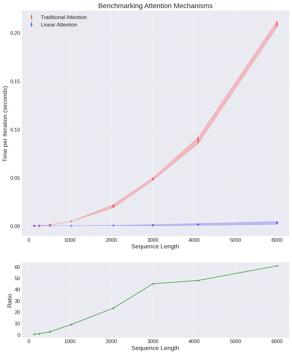
We’re going to to take a single attention layer, with a fixed d_k model dimension of 64, and benchmark the time taken for a forward pass of a 32 batch size set of sequences. The only variable to change will be the sequence length, spanning 128 up to 6000 (the GPT-3 context length for reference if 2048). Each run is done 100 times to get a mean and standard deviation, and experiments are run using an Nvidia T4 GPU.

For such a simple experiment the results are pretty striking.

The results show for even an incredibly small toy example that we get a speed up of up to 60x.

Discussion

There are a few obvious take-aways here:

1. The advantage of linear attention is huge — either in speed, higher throughput is always a good thing. Or in terms of memory requirements to process long sequences. In low memory environments this could be a big advantage.
2. The ratio plot has a surprising kink — leads us to suspect there’s some additional lower level optimisation happening here meaning the expected ratio doesn’t quite materalise. So we need to take this result with a pinch of salt.

For completeness also do not mistake this as saying “linear attention is 60x faster for small models”. In reality the feed-forward layers are often a bigger chunk of the parameters in a Transformer and the encoding / decoding is often a limiting size component as well. But in this tightly defined problem, pretty impressive!

Computational Complexity

If we think about the real time complexity of each approach we can show where this difference comes from.

Let’s break down the time complexity of the traditional softmax attention, the first term gives the complexity of QK multiplication which is n² scores, each a dot product of length d_k. The second term describes the complexity of the softmax on the attention scores, is in n². And the third term takes the n² matrix and dots it with the values vector.

If we assume for simplicity the query, key and vector matries have the same dimension we get the final term with the dominant n² term. (Provided the model dimension is << sequence length. )

The linear attention tells a different story. Again, if we look at the expression below for the time complexity we’ll analyse each of the terms.

The first term is the cost of applying the feature map to the Q and K matrices, the second term is the product between the Q and V matricies which results in a (d_k, d_v) matrix, and the K(QV) multiplication has the same complexity in the third term. Then the final output, again assuming the model dimensions are the same for the different matricies, gives a final complexity linear in sequence length, and quadratic in model dimension.

Therefore, so long as the model dimension is less than the sequence length we have a significantly faster model. The only real question left then is, how good an approximation is it anyway?

No free lunch — can we actually train a model?

Enough messing around, hopefully we’re all convinced that the linear attention is much faster than traditional attention so let’s do the real test. Can we actually train the models and do they perform similarly with the two different attention mechanisms?

The models we use here are really small — (and if there’s interest in a deeper dive into setting up a simple training harness we can look at that in the future) — and the data is simple. We’re just going to use the Penn Treebank dataset (publicly available through torchtext), which contains a collection of short snippets of text, which can be used to model / test small language models.

Can we train a real model to do real prediction

Real prediction might be a bit of a stretch here if we’re honest, given the number of parameters and time we’re training for all I’m really going to look for is do the training dynamics look similar. We’ll look at the loss curves for autoregressive training on a simple language modelling dataset, and if they follow the same shape we can at least have some confidence that the different mechanisms are giving us similar results.

The nature of the data means the outputs are rarely of high quality, but it gives all the trapping we’d expect of a proper training run.

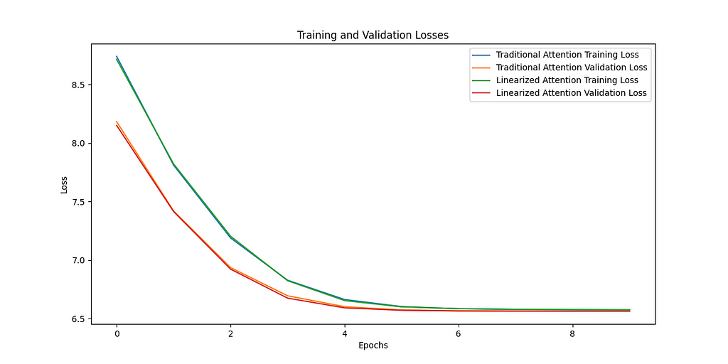
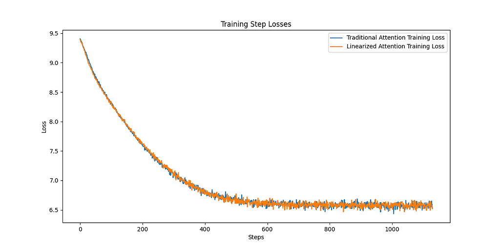
Let’s look at the training curves. The plot on the left shows the loss for training and validation for both the traditional and linear attention methods. We can see over the 10 epochs the two approaches are basically indistinguishable. Similarly if we look at the right plot, the loss for the traditional softmax and the linear attention is shown, again showing absolutely identical training dynamics.

Conclusion

This is obviously far from comprehensive, and we’re not exactly going to be competing with GPT here, but we can be pretty optimistic about reducing the complexity of the attention mechanism and not losing modelling ability.

Watch this space for a bigger comparison in Part 2.

All images, unless otherwise stated, have been created by the author, and the training data comes from the publicly available PennTreebank dataset accessed through PyTorch torchtext datasets. More details can be found here.

For more details on the implementation of linear attention I strongly recommend you look in more depth at the original paper (https://arxiv.org/abs/2006.16236) .

If you enjoyed this content follow this account or find me on Twitter.

Linear Attention Is All You Need was originally published in Towards Data Science on Medium, where people are continuing the conversation by highlighting and responding to this story.