Physics-Informed Neural Network with Forcing Function

Solving differential equations directly with neural networks (with code)

In physics, mathematics, economics, engineering, and many other fields, differential equations describe a function in terms of the derivatives of the variables. Put simply, when the rate of change of a variable in terms of other variables is involved, you will likely find a differential equation. Many examples describe these relationships. A differential equation’s solution is typically derived through analytical or numerical methods.

While deriving the analytic solution can be a tedious or, in some cases, an impossible task, a physics-informed neural network (PINN) produces the solution directly from the differential equation, bypassing the analytic process. This innovative approach to solving differential equations is an important development in the field.

A previous article by the author used a PINN to find the solution to a differential equation describing a simple electronic circuit. This article explores the more challenging task of finding a solution when driving the circuit with a forcing function. Consider the following series-connected electronic circuit that comprises a resistor R, capacitor C, inductor L, and a sinusoidal voltage source V sin(ωt). The behavior of the current flow, i(t), in this circuit is described by Equation 1, a 2nd-order non-homogeneous differential equation with forcing function, Vω/L cos(ωt).

Analytic solution

The analytic solution to Equation 1 requires solving the equation for three cases depending upon the relationship between λ and ω₀. As seen below, each results in a complicated and unique formula for i(t). In tests presented later in Results, these solutions will be compared against results produced by a PINN. The PINN will produce the solution directly from the differential equation without consideration of these cases.

(A detailed analytic solution by the author using Laplace transform techniques is available here.)

Case 1: Under-damped (λ/2 < ω₀)

Damping refers to how fast the circuit transitions from its starting transit to equilibrium. An under-damped response attempts to transition quickly but typically cycles through overshooting and undershooting before reaching equilibrium.

Case 2: Over-damped (λ/2 >ω₀)

An over-damped response slowly transitions from starting transit to equilibrium without undergoing cycles of overshooting and undershooting.

Case 3: Critically-damped (λ/2 = ω₀)

A critically-damped response falls between under-damped and over-damped, delivering the fastest response from starting transit to equilibrium.

PINN solution

PyTorch code is available here.

A neural network is typically trained with pairs of inputs and desired outputs. The inputs are applied to the neural network, and back-propagation adjusts the network’s weights and biases to minimize an objective function. The objective function represents the error in the neural network’s output compared to the desired output.

The objective function of a PINN, in contrast, requires three components: a residual component (obj ᵣₑₛ) and two initial condition components (obj ᵢₙᵢₜ₁ and obj ᵢₙᵢₜ₂). These are combined to produce the objective function:

Residual

The residual component is where physics-informed comes into play. This component, incorporating derivatives of the output, constrains the network to conform to the defining differential equation. The residual, Equation 6, is formed by rearranging Equation 1.

During training, values of t are presented to the neural network’s input, resulting in a residual. Backpropagation then reduces the residual component of the objective to a minimum value close to 0 over all the training points. The residual component is given by:

The first and second derivatives, di/dt and d²i/dt², required by Equation 6 are provided by the automatic differentiation function in the PyTorch and TensorFlow neural network platforms.

Initial condition 1

In this circuit example, the first initial condition requires that the PINN’s output, i(t) = 0 when input t = 0. This is due to the sinusoidal source V sin(t) = 0 at t = 0, resulting in no current flowing in the circuit. The objective component for initial condition 1 is given by Equation 8. During training, backpropagation will reduce this component to a value near 0.

Initial condition 2

The second initial condition requires that L di/dt = 0 when input t = 0. It is derived from Kirchhoff’s voltage law (i.e., the sum of voltage drops around a closed loop is zero). Specifically, at t = 0 the following conditions exist in the circuit:

• voltage source V sin(ωt) = 0
• capacitor C has an initial charge of Q = 0 , yielding a capacitor voltage of V_cap = Q/C = 0
• voltage across the resistor R is V_res = iR = 0, since i(t) = 0 (initial condition 1)
• voltage across the inductor L is V_ind = L di/dt
• given the above conditions, the sum of the voltage drops around the circuit reduces to L di/dt = 0

The objective component for initial condition 2 is given by Equation 9. Backpropagation will reduce this component to a value near 0.

Objective plot

The following figure shows the reduction in the value of the objective during training:

Results

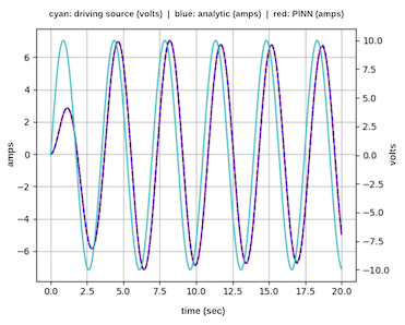
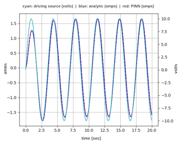
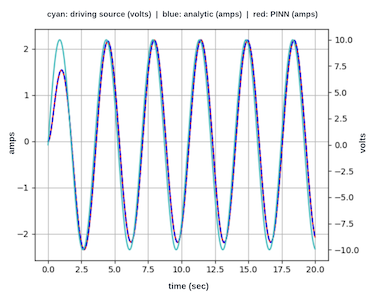
The following test cases compare the response of the trained PINN to the appropriate analytic solution for each case. The circuit component values were chosen to produce the conditions of under-damped, overdamped, and critically-damped responses, as discussed above. All three cases are driven with a sinusoidal voltage source of V = 10 volts and ω = 1.8 radians/second. For each case, the capacitor and inductor values are C = 0.3 farads and L = 1.51 henries, respectively. The value of the resistor R is noted below for each case.

Under-damped
(R = 1.2 ohms)

Over-damped
(R = 6.0 ohms)

Critically-damped
(R = 4.487 ohms)

Conclusion

In this article, a neural network with a custom objective function was used to successfully solve a differential equation describing an electronic circuit driven by a sinusoidal source. Typically, the solution to a differential equation is derived through a tedious analytic process or numerically. The example presented here demonstrates that a neural network can accurately solve these equations in a straightforward and efficient manner. As shown in the three test cases, the neural network response is identical to the analytic solution.

Appendix: PINN training notes

• PINN structure:
  – input layer, 1 input
  – hidden layer, 128 neurons with GELU activation
  – hidden layer, 128 neurons with GELU activation
  – output layer, 1 neuron with linear activation
• The PINN is trained with 220 points in the time domain of 0 to 20 seconds. The number of points is controlled by the duration of the domain and a hyperparameter for the number of points per second, which is set to 11 points/sec for the test cases. This value gives a sufficient number of training points for each period of a sinusoidal driving source with ω = 1.8. For higher values of ω, more points per second are required, e.g., ω = 4.0 requires 25 points/sec.
• The PINN is trained in batches of 32 points sampled from the set of all training points. The training points are randomly shuffled at every epoch.
• The learning rate starts at a value of 0.01 at the beginning of training and decreases by factor of 0.75 every 2000 epochs.
• The objective plot is an important indicator of successful training. As training progresses, the objective should decrease by several orders of magnitude and bottom out at a small value near 0. If training fails to produce this result, the hyperparameters will require adjustment. It is recommended to first try increasing the number of epochs and then increasing the number of training points per second.

A pdf of this article is available here.

All images, unless otherwise noted, are by the author.

Physics-Informed Neural Network with Forcing Function was originally published in Towards Data Science on Medium, where people are continuing the conversation by highlighting and responding to this story.