Feature Selection with Optuna

A versatile and promising approach for the feature selection task

Feature selection is a critical step in many machine learning pipelines. In practice, we generally have a wide range of variables available as predictors for our models, but only a few of them are related to our target. Feature selection consists of finding a reduced set of these features, mainly for:

• Improved generalization — using a reduced number of features minimizes the risk of overfitting.
• Better inference — by removing redundant features (for example, two features very correlated with each other), we can retain only one of them and better capture its effect.
• Efficient training — having less features means shorter training times.
• Better interpretation — reducing the number of features produces more parsimonious models which are easier to understand.

There are many techniques available to perform feature selection, each with varying complexity. In this article, I want to share a way of using a powerful open source optimization tool, Optuna, to perform the feature selection task in an innovative way. The main idea is to have a flexible tool that can handle feature selection for a wide range of tasks, by efficiently testing different feature combinations (e.g., not trying them all one by one). Below, we’ll go through a hands-on example implementing this approach, and also comparing it to other common feature selection strategies. To experiment with the feature selection techniques discussed, you can follow along with this Colab Notebook.

In this example, we’ll focus on a classification task based on the Mobile Price Classification dataset from Kaggle. We have 20 features, including ‘battery_power’, ‘clock_speed’ and ‘ram’, to predict the ‘price_range’ feature, which can belong to four different bands: 0, 1, 2 and 3.

We first split our dataset into train and test sets, and we also prepare a 5-fold validation split within the train set — this will be useful later on.

import pandas as pd
from sklearn.model_selection import train_test_split
from sklearn.model_selection import StratifiedKFold

SEED = 32

# Load data
filename = "train.csv" # train.csv from https://www.kaggle.com/datasets/iabhishekofficial/mobile-price-classification

df = pd.read_csv(filename)

# Train - test split
df_train, df_test = train_test_split(df, test_size=0.2, stratify=df.iloc[:,-1], random_state=SEED)
df_train = df_train.reset_index(drop=True)
df_test = df_test.reset_index(drop=True)

# The last column is the target variable
X_train = df_train.iloc[:,0:20]
y_train = df_train.iloc[:,-1]
X_test = df_test.iloc[:,0:20]
y_test = df_test.iloc[:,-1]

# Stratified kfold over the train set for cross validation
skf = StratifiedKFold(n_splits=5, shuffle=True, random_state=SEED)
splits = list(skf.split(X_train, y_train))

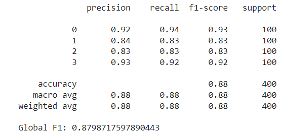
The model we’ll use throughout the example is the Random Forest Classifier, using the scikit-learn implementation and default parameters. We first train the model using all features to set our benchmark. The metric we’ll measure is the F1 score weighted for all four price ranges. After fitting the model over the train set, we evaluate it on the test set, obtaining an F1 score of around 0.87.

from sklearn.ensemble import RandomForestClassifier
from sklearn.metrics import f1_score, classification_report

model = RandomForestClassifier(random_state=SEED)
model.fit(X_train,y_train)
preds = model.predict(X_test)

print(classification_report(y_test, preds))
print(f"Global F1: {f1_score(y_test, preds, average='weighted')}")

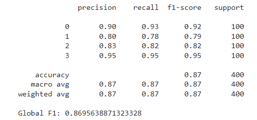
The goal now is to improve these metrics by selecting a reduced feature set. We will first outline how our Optuna-based approach works, and then test and compare it with other common feature selection strategies.

Optuna

Optuna is an optimization framework mainly used for hyperparameter tuning. One of the key features of the framework is its use of Bayesian optimization techniques to search the parameter space. The main idea is that Optuna tries different combinations of parameters and evaluates how the objective function changes with each configuration. From these trials, it builds a probabilistic model used to estimate which parameter values are likely to yield better outcomes.

This strategy is much more efficient compared to grid or random search. For example, if we had n features, and attempted to try each possible feature subset, we would have to perform 2^n trials. With 20 features these would be more than a million trials. Instead, with Optuna, we can explore the search space with much fewer trials.

Optuna offers various samplers to try. For our case, we’ll use the default one, the TPESampler, based on the Tree-structured Parzen Estimator algorithm (TPE). This sampler is the most commonly used, and it’s recommended for searching categorical parameters, which is our case as we’ll see below. According to the documentation, this algorithm “fits one Gaussian Mixture Model (GMM) l(x) to the set of parameter values associated with the best objective values, and another GMM g(x) to the remaining parameter values. It chooses the parameter value x that maximizes the ratio l(x)/g(x).”

As mentioned earlier, Optuna is typically used for hyperparameter tuning. This is usually done by training the model repeatedly on the same data using a fixed set of features, and in each trial testing a new set of hyperparameters determined by the sampler. The parameter set that minimizes the given objective function is then returned as the best trial.

In our case, however, we’ll use a fixed model with predetermined parameters, and in each trial, we’ll allow Optuna to select which features to try. The process aims to find the set of features that minimizes the loss function. In our case, we’ll guide the algorithm to maximize the F1 score (or minimize the negative of the F1). Additionally, we’ll add a small penalty for each feature used, to encourage smaller feature sets (if two feature sets yield similar results, we’ll prefer the one with fewer features).

The data we’ll use is the train dataset, split into five folds. In each trial, we’ll fit the classifier five times using four of the five folds for training and the remaining fold for validation. We’ll then average the validation metrics and add the penalty term to calculate the trial’s loss.

Below is the implemented class to perform the feature selection search:

import optuna

class FeatureSelectionOptuna:
    """
    This class implements feature selection using Optuna optimization framework.

    Parameters:

    - model (object): The predictive model to evaluate; this should be any object that implements fit() and predict() methods.
    - loss_fn (function): The loss function to use for evaluating the model performance. This function should take the true labels and the
                          predictions as inputs and return a loss value.
    - features (list of str): A list containing the names of all possible features that can be selected for the model.
    - X (DataFrame): The complete set of feature data (pandas DataFrame) from which subsets will be selected for training the model.
    - y (Series): The target variable associated with the X data (pandas Series).
    - splits (list of tuples): A list of tuples where each tuple contains two elements, the train indices and the validation indices.
    - penalty (float, optional): A factor used to penalize the objective function based on the number of features used.
    """

    def __init__(self,
                 model,
                 loss_fn,
                 features,
                 X,
                 y,
                 splits,
                 penalty=0):

        self.model = model
        self.loss_fn = loss_fn
        self.features = features
        self.X = X
        self.y = y
        self.splits = splits
        self.penalty = penalty

    def __call__(self,
                 trial: optuna.trial.Trial):

        # Select True / False for each feature
        selected_features = [trial.suggest_categorical(name, [True, False]) for name in self.features]

        # List with names of selected features
        selected_feature_names = [name for name, selected in zip(self.features, selected_features) if selected]

        # Optional: adds a penalty for the amount of features used
        n_used = len(selected_feature_names)
        total_penalty = n_used * self.penalty

        loss = 0

        for split in self.splits:
          train_idx = split[0]
          valid_idx = split[1]

          X_train = self.X.iloc[train_idx].copy()
          y_train = self.y.iloc[train_idx].copy()
          X_valid = self.X.iloc[valid_idx].copy()
          y_valid = self.y.iloc[valid_idx].copy()

          X_train_selected = X_train[selected_feature_names].copy()
          X_valid_selected = X_valid[selected_feature_names].copy()

          # Train model, get predictions and accumulate loss
          self.model.fit(X_train_selected, y_train)
          pred = self.model.predict(X_valid_selected)

          loss += self.loss_fn(y_valid, pred)

        # Take the average loss across all splits
        loss /= len(self.splits)

        # Add the penalty to the loss
        loss += total_penalty

        return loss

The key part is where we define which features to use. We treat each feature as one parameter, which can take the values True or False. These values indicate whether the feature should be included in the model. We use the suggest_categorical method so that Optuna selects one of the two possible values for each feature.

We now initialize our Optuna study and perform the search for 100 trials. Notice that we enqueue a first trial using all features, as a starting point for the search, allowing Optuna to compare subsequent trials against a fully-featured model:

from optuna.samplers import TPESampler

def loss_fn(y_true, y_pred):
  """
  Returns the negative F1 score, to be treated as a loss function.
  """
  res = -f1_score(y_true, y_pred, average='weighted')
  return res

features = list(X_train.columns)

model = RandomForestClassifier(random_state=SEED)

sampler = TPESampler(seed = SEED)
study = optuna.create_study(direction="minimize",sampler=sampler)

# We first try the model using all features
default_features = {ft: True for ft in features}
study.enqueue_trial(default_features)

study.optimize(FeatureSelectionOptuna(
                         model=model,
                         loss_fn=loss_fn,
                         features=features,
                         X=X_train,
                         y=y_train,
                         splits=splits,
                         penalty = 1e-4,
                         ), n_trials=100)

After completing the 100 trials, we retrieve the best one from the study and the features used in it. These are the following:

[‘battery_power’, ‘blue’, ‘dual_sim’, ‘fc’, ‘mobile_wt’, ‘px_height’, ‘px_width’, ‘ram’, ‘sc_w’]

Notice that from the original 20 features, the search concluded with only 9 of them, which is a significant reduction. These features yielded a minimum validation loss of around -0.9117, which means they achieved an average F1 score of around 0.9108 across all folds (after adjusting for the penalty term).

The next step is to train the model on the entire train set using these selected features and evaluate it on the test set. This results in an F1 score of around 0.882:

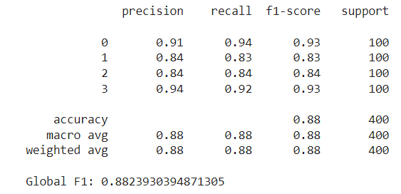
By selecting the right features, we were able to reduce our feature set by more than half, while still achieving a higher F1 score than with the full set. Below we will discuss some pros and cons of using Optuna for feature selection:

Pros:

• Searches across feature sets efficiently, taking into account which feature combinations are most likely to produce good results.
• Adaptable for many scenarios: As long as there is a model and a loss function, we can use it for any feature selection task.
• Sees the whole picture: Unlike methods that evaluate features individually, Optuna takes into account which features tend to go well with each other, and which don’t.
• Dynamically determines the number of features as part of the optimization process. This can be tuned with the penalty term.

Cons:

• It’s not as straightforward as simpler methods, and for smaller and simpler datasets it might not be worth it.
• Although it requires much fewer trials than other methods (like exhaustive search), it still typically requires around 100 to 1000 trials. Depending on the model and dataset, this can be time-consuming and computationally expensive.

Next, we’ll compare our approach to other common feature selection strategies.

Other Methods

Filter Methods — Chi-Squared

One of the simplest alternatives is to evaluate each feature individually using a statistial test and retain the top k features based on their scores. Notice that this approach doesn’t require any machine learning model. For example, for the classification task, we can choose the chi-squared test, which determines whether there is a statistically significant association between each feature and the target variable. We’ll use the SelectKBest class from scikit-learn, which applies the score function (chi-squared) to each feature and returns the top k scoring variables. Unlike the Optuna method, the number of features isn’t determined in the selection process, but must be set beforehand. In this case, we’ll set this number at ten. These methods fall within the filter methods class. They tend to be the easiest and fastest to compute since they don’t require any model behind.

from sklearn.feature_selection import SelectKBest, chi2

skb = SelectKBest(score_func=chi2, k=10)
skb.fit(X_train,y_train)

scores = pd.DataFrame(skb.scores_)
cols = pd.DataFrame(X_train.columns)
featureScores = pd.concat([cols,scores],axis=1)
featureScores.columns = ['feature','score']
featureScores.nlargest(10, 'score')

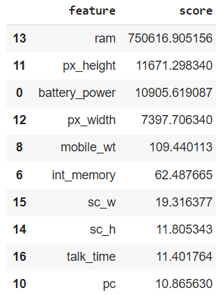
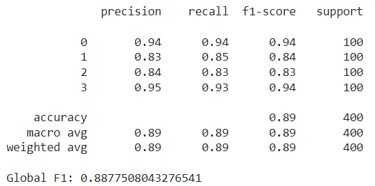
In our case, ram scored the highest by far in the chi-squared test, followed by px_height and battery_power. Notice that these features were also selected by our Optuna method above, along with px_width, mobile_wt and sc_w. However, there are some new additions like int_memory and talk_time — these weren’t picked by the Optuna study. After training the random forest with these 10 features and evaluating it on the test set, we achieved an F1 score slightly higher than our previous best, at approximately 0.888:

Pros:

• Model agnostic: doesn’t require a machine learning model.
• Easy and fast to implement and run.

Cons:

• It has to be adapted for each task. For instance, some score functions are only applicable for classification tasks, and others only for regression tasks.
• Greedy: depending on the alternative used, it usually looks at features one by one, without taking into account which are already included in the set.
• Requires the number of features to select to be set beforehand.

Wrapper Methods — Forward Search

Wrapper methods are another class of feature selection strategies. These are iterative methods; they involve training the model with a set of features, evaluating its performance, and then deciding whether to add or remove features. Our Optuna strategy falls within these methods. However, most common examples include forward selection or backward selection. With forward selection, we begin with no features and, at each step, we greedily add the feature that provides the highest performance gain, until a stop criterion is met (number of features or performance decline). Conversely, backward selection starts with all features and iteratively removes the least significant ones at each step.

Below, we try the SequentialFeatureSelector class from scikit-learn, performing a forward selection until we find the top 10 features. This method will also make use of the 5-fold split we performed above, averaging performance across the validation splits at each step.

from sklearn.feature_selection import SequentialFeatureSelector

model = RandomForestClassifier(random_state=SEED)
sfs = SequentialFeatureSelector(model, n_features_to_select=10, cv=splits)
sfs.fit(X_train, y_train);

selected_features = list(X_train.columns[sfs.get_support()])
print(selected_features)

This method ends up selecting the following features:

[‘battery_power’, ‘blue’, ‘fc’, ‘mobile_wt’, ‘px_height’, ‘px_width’, ‘ram’, ‘talk_time’, ‘three_g’, ‘touch_screen’]

Again, some are common to the previous methods, and some are new (e.g., three_g and touch_screen. Using these features, the Random Forest achieves a lower test F1 score, slightly below 0.88.

Pros

• Easy to implement in just a few lines of code.
• It can also be used to determine the number of features to use (using the tolerance parameter).

Cons

• Time consuming: Starting with zero features, it trains the model each time using a different variable, and retains the best one. For the next step, it again tries out all features (now including the previous one), and again selects the best one. This is repeated until the desired number of features is reached.
• Greedy: Once a feature is included, it stays. This may lead to suboptimal results, as the feature providing the highest individual gain in early rounds might not be the best choice in the context of other feature interactions.

Feature Importance

Finally, we’ll explore another straightforward selection strategy, which involves using the feature importances the model learns (if available). Certain models, like Random Forests, provide a measure of which features are most important for prediction. We can use these rankings to filter out those features that, according to the model, have the least importance. In this case, we train the model on the entire train dataset, and retain the 10 most important features:

model = RandomForestClassifier(random_state=SEED)
model.fit(X_train,y_train)

importance = pd.DataFrame({'feature':X_train.columns, 'importance':model.feature_importances_})
importance.nlargest(10, 'importance')

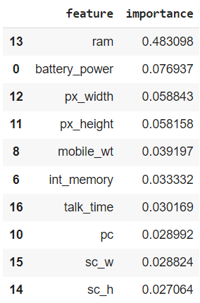
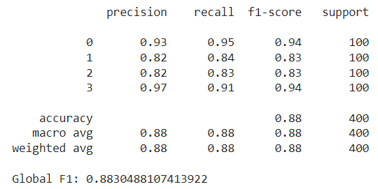
Notice how, once again, ram is ranked highest, far above the second most important feature. Training with these 10 features, we obtain a test F1 score of almost 0.883, similar to the ones we’ve been seeing. Also, note how the features selected through feature importance are the same as those selected using the chi-squared test, although they are ranked differently. This difference in ranking results in a slightly different outcome.

Pros:

• Easy and fast to implement: it requires a single training of the model and directly uses the derived feature importances.
• It can be adapted into a recursive version, in which at each step the least important feature is removed and the model is then trained again (see Recursive Feature Elimination).
• Contained within the model: If the model we are using provides feature importances, we already have a feature selection alternative available at no additional cost.

Cons:

• Feature importance might not be aligned with our end goal. For instance, a feature might appear unimportant on its own but could be critical due to its interaction with other features. Also, an important feature might be counterproductive overall, by affecting the performance of other useful predictors.
• Not all models offer feature importance estimation.
• Requires the number of features to select to be predefined.

Closing Remarks

To conclude, we’ve seen how to use Optuna, a powerful optimization tool, for the feature selection task. By efficiently navigating the search space, it is able to find good feature subsets with relatively few trials. Not only that, but it is also flexible and can be adapted to many scenarios as long as we have a model and a loss function defined.

Throughout our examples, we observed that all techniques yielded similar feature sets and results. This is mainly because the dataset we used is rather simple. In these cases, simpler methods already produce a good feature selection, so it wouldn’t make much sense to go with the Optuna approach. However, for more complex datasets, with more features and intricate relationships between them, using Optuna might be a good idea. So, all in all, given its relative ease of implementation and ability to deliver good results, using Optuna for feature selection is a worthwhile addition to the data scientist’s toolkit.

Thanks for reading!

Colab Notebook: https://colab.research.google.com/drive/193Jwb0xXWh_UkvwIiFgufKEYer-86RNA?usp=sharing

Feature Selection with Optuna was originally published in Towards Data Science on Medium, where people are continuing the conversation by highlighting and responding to this story.