Understand SQL Window Functions Once and For All

A step-by-step guide to understanding window functions

Window functions are key to writing SQL code that is both efficient and easy to understand. Knowing how they work and when to use them will unlock new ways of solving your reporting problems.

The objective of this article is to explain window functions in SQL step by step in an understandable way so that you don’t need to rely on only memorizing the syntax.

Here is what we will cover:

• An explanation on how you should view window functions
• Go over many examples in increasing difficulty
• Look at one specific real-case scenario to put our learnings into practice
• Review what we’ve learned

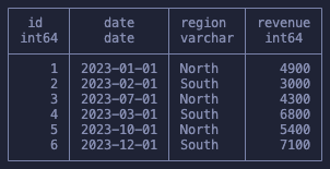
Our dataset is simple, six rows of revenue data for two regions in the year 2023.

Window Functions Are Sub Groups

If we took this dataset and ran a GROUP BY sum on the revenue of each region, it would be clear what happens, right? It would result in only two remaining rows, one for each region, and then the sum of the revenues:

The way I want you to view window functions is very similar to this but, instead of reducing the number of rows, the aggregation will run “in the background” and the values will be added to our existing rows.

First, an example:

SELECT
 id,
    date,
    region,
    revenue,
    SUM(revenue) OVER () as total_revenue
FROM
    sales

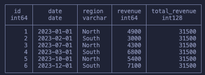
Notice that we don’t have any GROUP BY and our dataset is left intact. And yet we were able to get the sum of all revenues. Before we go more in depth in how this worked let’s just quickly talk about the full syntax before we start building up our knowledge.

The Window Function Syntax

The syntax goes like this:

SUM([some_column]) OVER (PARTITION BY [some_columns] ORDER BY [some_columns])

Picking apart each section, this is what we have:

• An aggregation or window function: SUM, AVG, MAX, RANK, FIRST_VALUE
• The OVER keyword which says this is a window function
• The PARTITION BY section, which defines the groups
• The ORDER BY section which defines if it’s a running function (we will cover this later on)

Don’t stress over what each of these means yet, as it will become clear when we go over the examples. For now just know that to define a window function we will use the OVER keyword. And as we saw in the first example, that’s the only requirement.

Building Our Understanding Step By Step

Moving to something actually useful, we will now apply a group in our function. The initial calculation will be kept to show you that we can run more than one window function at once, which means we can do different aggregations at once in the same query, without requiring sub-queries.

SELECT
    id,
    date,
    region,
    revenue,
    SUM(revenue) OVER (PARTITION BY region) as region_total,
    SUM(revenue) OVER () as total_revenue
FROM sales

As said, we use the PARTITION BY to define our groups (windows) that are used by our aggregation function! So, keeping our dataset intact we’ve got:

• The total revenue for each region
• The total revenue for the whole dataset

We’re also not restrained to a single group. Similar to GROUP BY we can partition our data on Region and Quarter, for example:

SELECT
    id,
    date,
    region,
    revenue,
    SUM(revenue) OVER (PARTITION BY 
          region, 
          date_trunc('quarter', date)
    ) AS region_quarterly_revenue
FROM sales

In the image we see that the only two data points for the same region and quarter got grouped together!

At this point I hope it’s clear how we can view this as doing a GROUP BY but in-place, without reducing the number of rows in our dataset. Of course, we don’t always want that, but it’s not that uncommon to see queries where someone groups data and then joins it back in the original dataset, complicating what could be a single window function.

Moving on to the ORDER BY keyword. This one defines a running window function. You’ve probably heard of a Running Sum once in your life, but if not, we should start with an example to make everything clear.

SELECT
    id,
    date,
    region,
    revenue,
    SUM(revenue) OVER (ORDER BY id) as running_total
FROM sales

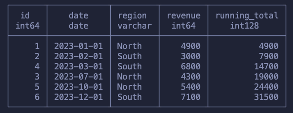
What happens here is that we’ve went, row by row, summing the revenue with all previous values. This was done following the order of the id column, but it could’ve been any other column.

This specific example is not particularly useful because we’re summing across random months and two regions, but using what we’ve learned we can now find the cumulative revenue per region. We do that by applying the running sum within each group.

SELECT
    id,
    date,
    region,
    revenue,
    SUM(revenue) OVER (PARTITION BY region ORDER BY date) as running_total
FROM sales

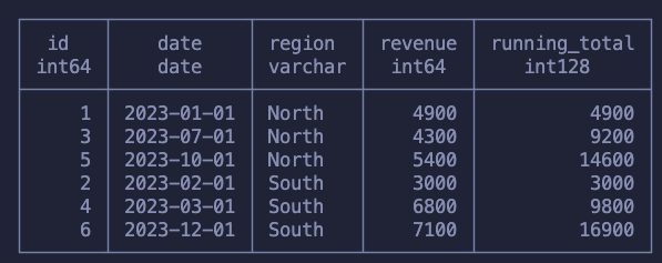
Take the time to make sure you understand what happened here:

• For each region we’re walking up month by month and summing the revenue
• Once it’s done for that region we move to the next one, starting from scratch and again moving up the months!

It’s quite interesting to notice here that when we’re writing these running functions we have the “context” of other rows. What I mean is that to get the running sum at one point, we must know the previous values for the previous rows. This becomes more obvious when we learn that we can manually chose how many rows before/after we want to aggregate on.

SELECT
    id,
    date,
    region,
    revenue,
    SUM(revenue) OVER (ORDER BY id ROWS BETWEEN 1 PRECEDING AND 2 FOLLOWING) 
    AS useless_sum
FROM
    sales

For this query we specified that for each row we wanted to look at one row behind and two rows ahead, so that means we get the sum of that range! Depending on the problem you’re solving this can be extremely powerful as it gives you complete control on how you’re grouping your data.

Finally, one last function I want to mention before we move into a harder example is the RANK function. This gets asked a lot in interviews and the logic behind it is the same as everything we’ve learned so far.

SELECT
    *,
    RANK() OVER (PARTITION BY region ORDER BY revenue DESC) as rank,
    RANK() OVER (ORDER BY revenue DESC) as overall_rank
FROM
    sales
ORDER BY region, revenue DESC

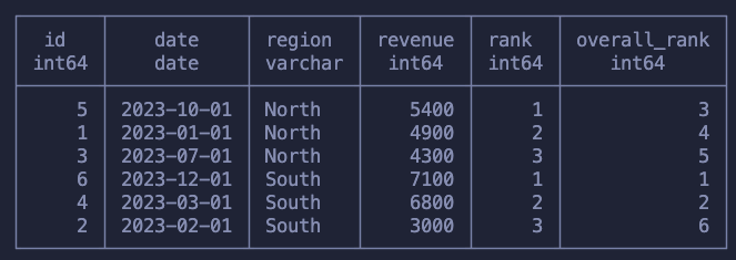
Just as before, we used ORDER BY to specify the order which we will walk, row by row, and PARTITION BY to specify our sub-groups.

The first column ranks each row within each region, meaning that we will have multiple “rank one’s” in the dataset. The second calculation is the rank across all rows in the dataset.

Forward Filling Missing Data

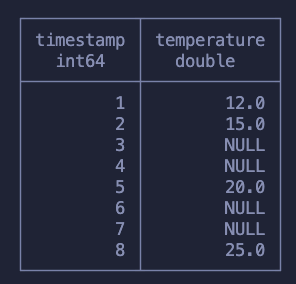
This is a problem that shows up every now and then and to solve it on SQL it takes heavy usage of window functions. To explain this concept we will use a different dataset containing timestamps and temperature measurements. Our goal is to fill in the rows missing temperature measurements with the last measured value.

Here is what we expect to have at the end:

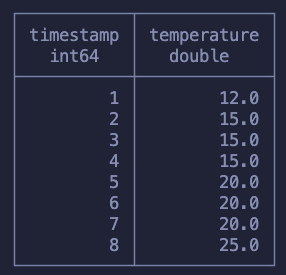
Before we start I just want to mention that if you’re using Pandas you can solve this problem simply by running df.ffill() but if you’re on SQL the problem gets a bit more tricky.

The first step to solve this is to, somehow, group the NULLs with the previous non-null value. It might not be clear how we do this but I hope it’s clear that this will require a running function. Meaning that it’s a function that will “walk row by row”, knowing when we hit a null value and when we hit a non-null value.

The solution is to use COUNT and, more specifically, count the values of temperature measurements. In the following query I run both a normal running count and also a count over the temperature values.

SELECT
    *,
    COUNT() OVER (ORDER BY timestamp) as normal_count,
    COUNT(temperature) OVER (ORDER BY timestamp) as group_count
from sensor

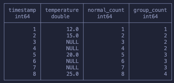
• In the first calculation we simply counted up each row increasingly
• On the second one we counted every value of temperature we saw, not counting when it was NULL

The normal_count column is useless for us, I just wanted to show what a running COUNT looked like. Our second calculation though, the group_count moves us closer to solving our problem!

Notice that this way of counting makes sure that the first value, just before the NULLs start, is counted and then, every time the function sees a null, nothing happens. This makes sure that we’re “tagging” every subsequent null with the same count we had when we stopped having measurements.

Moving on, we now need to copy over the first value that got tagged into all the other rows within that same group. Meaning that for the group 2 needs to all be filled with the value 15.0.

Can you think of a function now that we can use here? There is more than one answer for this, but, again, I hope that at least it’s clear that now we’re looking at a simple window aggregation with PARTITION BY .

SELECT
    *,
    FIRST_VALUE(temperature) OVER (PARTITION BY group_count) as filled_v1,
    MAX(temperature) OVER (PARTITION BY group_count) as filled_v2
FROM (
    SELECT
        *,
        COUNT(temperature) OVER (ORDER BY timestamp) as group_count
    from sensor
) as grouped
ORDER BY timestamp ASC

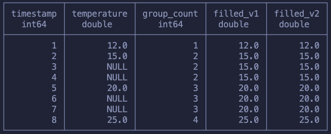
We can use both FIRST_VALUE or MAX to achieve what we want. The only goal is that we get the first non-null value. Since we know that each group contains one non-null value and a bunch of null values, both of these functions work!

This example is a great way to practice window functions. If you want a similar challenge try to add two sensors and then forward fill the values with the previous reading of that sensor. Something similar to this:

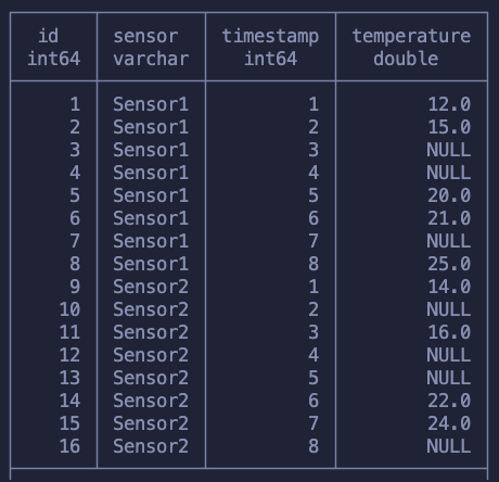
Could you do it? It doesn’t use anything that we haven’t learned here so far.

By now we know everything that we need about how window functions work in SQL, so let’s just do a quick recap!

Recap Time

This is what we’ve learned:

• We use the OVER keyword to write window functions
• We use PARTITION BY to specify our sub-groups (windows)
• If we provide only the OVER() keyword our window is the whole dataset
• We use ORDER BY when we want to have a running function, meaning that our calculation walks row by row
• Window functions are useful when we want to group data to run an aggregation but we want to keep our dataset as is

I hope this helped you understand how window functions work and helps you apply it in the problems you need to solve.

All images by the author unless stated otherwise

Understand SQL Window Functions Once and For All was originally published in Towards Data Science on Medium, where people are continuing the conversation by highlighting and responding to this story.