Transform Data with Hyperbolic Sine

Why handling negative values should be a cinch

Many models are sensitive to outliers, such as linear regression, k-nearest neighbor, and ARIMA. Machine learning algorithms suffer from over-fitting and may not generalize well in the presence of outliers.¹ However, the right transformation can shrink these extreme values and improve your model’s performance.

Transformations for data with negative values include:

1. Shifted Log
2. Shifted Box-Cox
3. Inverse Hyperbolic Sine
4. Sinh-arcsinh

Log and Box-Cox are effective tools when working with positive data, but inverse hyperbolic sine (arcsinh) is much more effective on negative values.

Sinh-arcsinh is even more powerful. It has two parameters that can adjust the skew and kurtosis of your data to make it close to normal. These parameters can be derived using gradient descent. See an implementation in python at the end of this post.

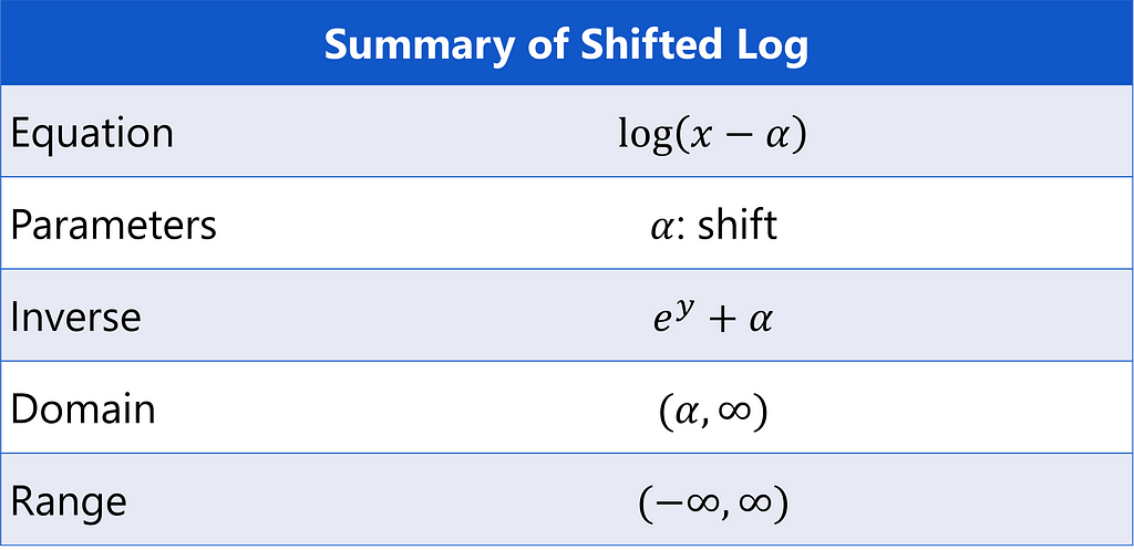
Shifted Log

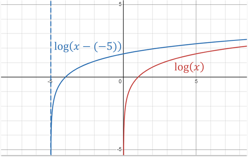
The log transformation can be adapted to handle negative values with a shifting term α.

Visually, this is moving the log’s vertical asymptote from 0 to α.

Forecasting Stock Prices

Imagine you are a building a model to predict the stock market. Hosenzade and Haratizadeh tackle this problem with a convolutional neural network using a large set of feature variables that I have pulled from UCI Irvine Machine Learning Repository². Below is distribution of the change of volume feature — an important technical indicator for stock market forecasts.

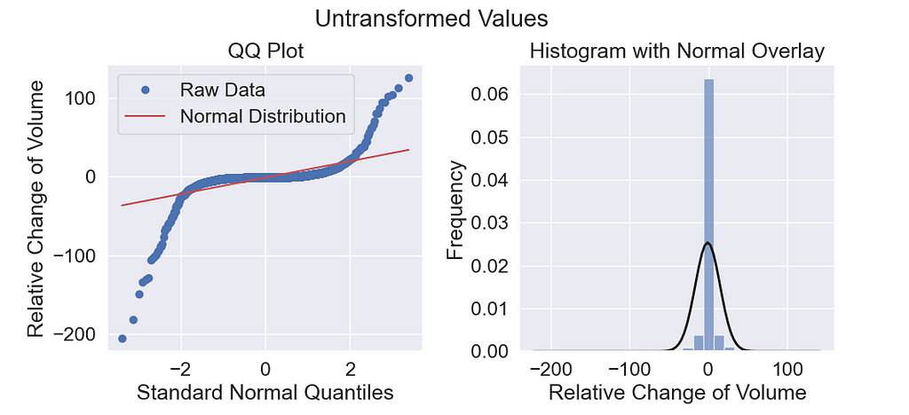
The quantile-quantile (QQ) plot reveals heavy right and left tails. The goal of our transformation will be to bring the tails closer to normal (the red line) so that it has no outliers.

Using a shift value of -250, I get this log distribution.

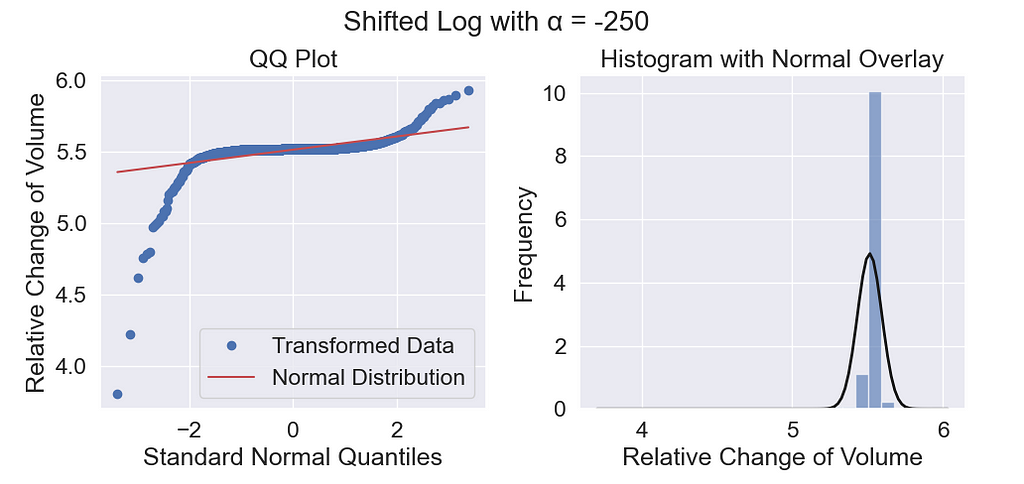
The right tail looks a little better, but the left tail still shows deviation from the red line. Log works by applying a concave function to the data which skews the data left by compressing the high values and stretching out the low values.

The log transformation only makes the right tail lighter.

While this works well for positively skewed data, it is less effective for data with negative outliers.

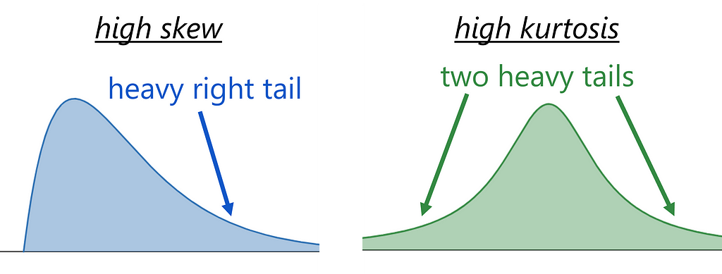
In the stock data, skewness is not the issue. The extreme values are on both left and right sides. The kurtosis is high, meaning that both tails are heavy. A simple concave function is not equipped for this situation.

Shifted Box-Cox

Box-Cox is a generalized version of log, which can also be shifted to include negative values, written as

The λ parameter controls the concavity of the transformation allowing it to take on a variety of forms. Box-cox is quadratic when λ = 2. It’s linear when λ = 1, and log as λ approaches 0. This can be verified by using L’Hôpital’s rule.

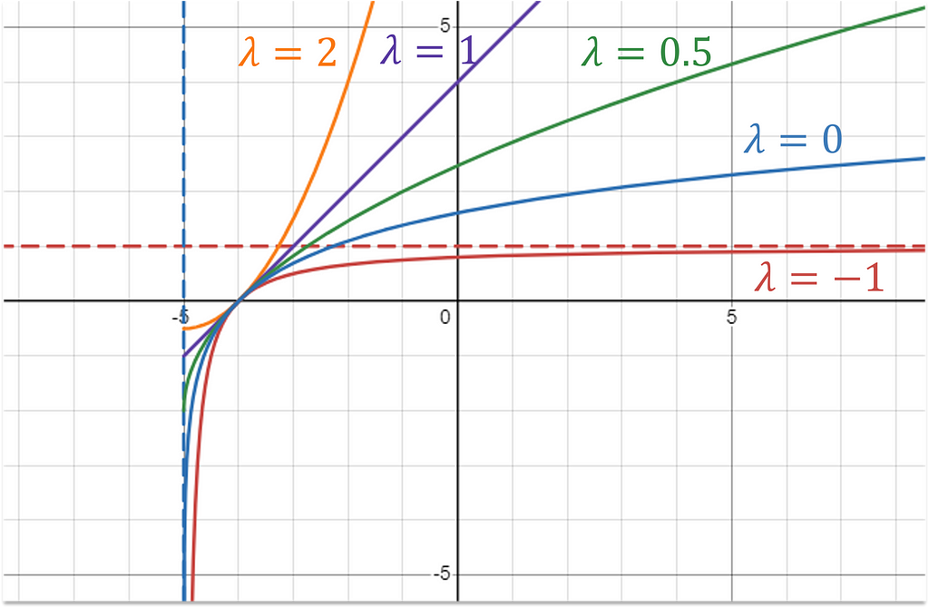
To apply this transformation on our stock price data, I use a shift value -250 and determine λ with scipy’s boxcox function.

from scipy.stats import boxcox
y, lambda_ = boxcox(x - (-250))

The resulting transformed data looks like this:

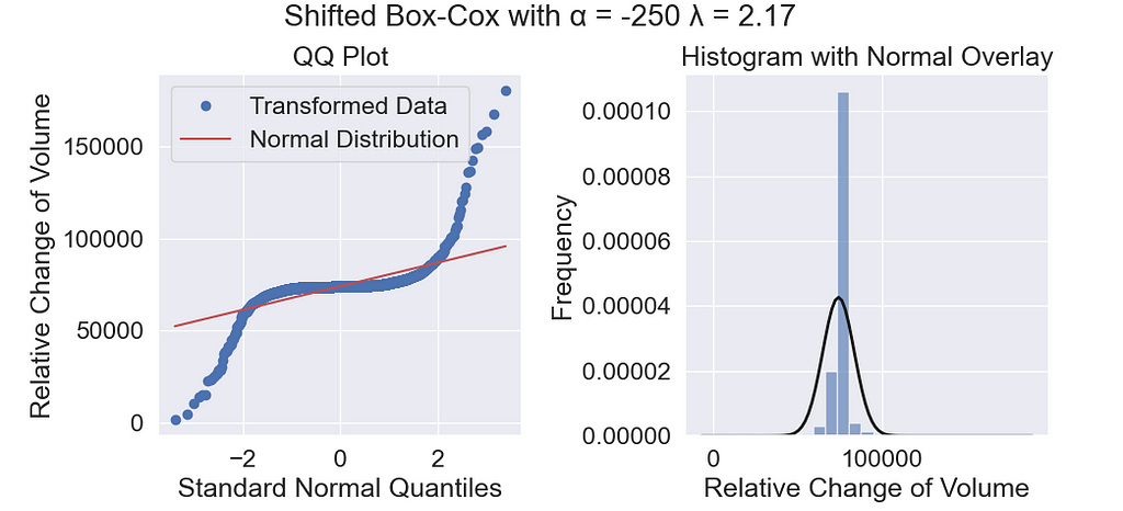
Despite the flexibility of this transformation, it fails to reduce the tails on the stock price data. Low values of λ skew the data left, shrinking the right tail. High values of λ skew the data right, shrinking the left tail, but there isn’t any value that can shrink both simultaneously.

Inverse Hyperbolic Sine

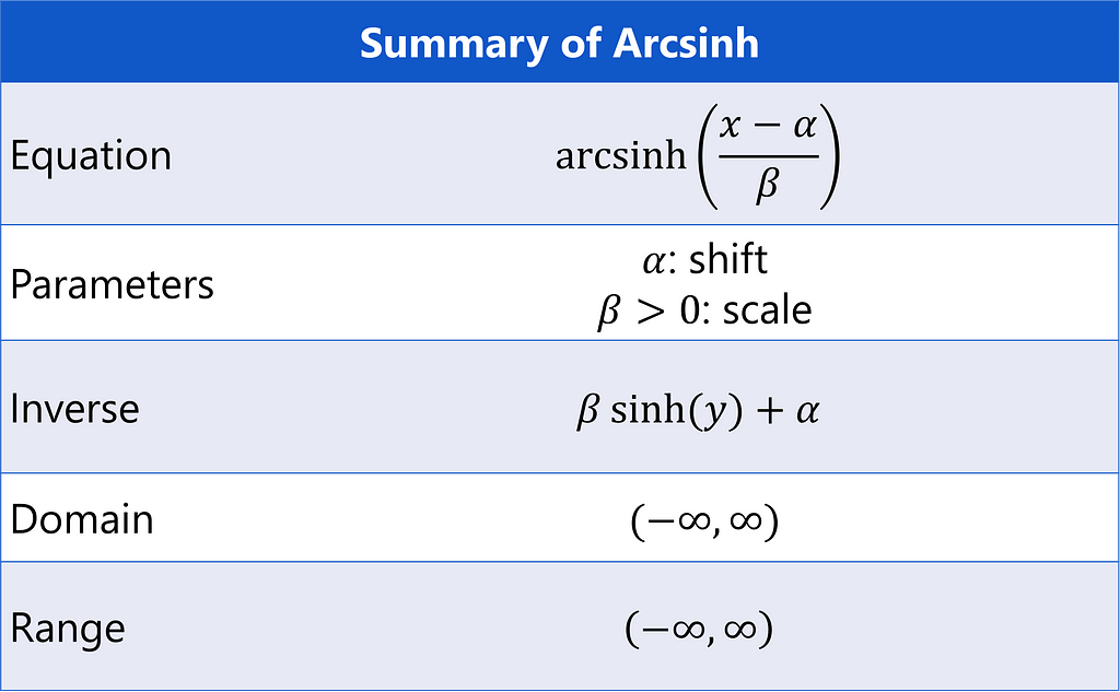
The hyperbolic sine function (sinh) is defined as

and its inverse is

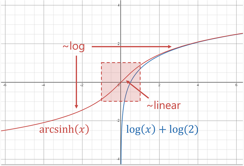
In this case, the inverse is a more helpful function because it’s approximately log for large x (positive or negative) and linear for small values of x. In effect, this shrinks extremes while keeping the central values, more or less, the same.

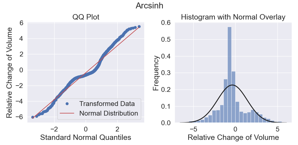
Arcsinh reduces both positive and negative tails.

For positive values, arcsinh is concave, and for negative values, it’s convex. This change in curvature is the secret sauce that allows it to handle positive and negative extreme values simultaneously.

Using this transformation on the stock data results in near normal tails. The new data has no outliers!

Scale Matters

Consider how your data is scaled before it’s passed into arcsinh.

For log, your choice of units is irrelevant. Dollars or cents, grams or kilograms, miles or feet —it’s all the same to the log function. The scale of your inputs only shifts the transformed values by a constant value.

The same is not true for arcsinh. Values between -1 and 1 are left almost unchanged while large numbers are log-dominated. You may need to play around with different scales and offsets before feeding your data into arcsinh to get a result you are satisfied with.

At the end of the article, I implement a gradient descent algorithm in python to estimate these transformation parameters more precisely.

Sinh-arcsinh

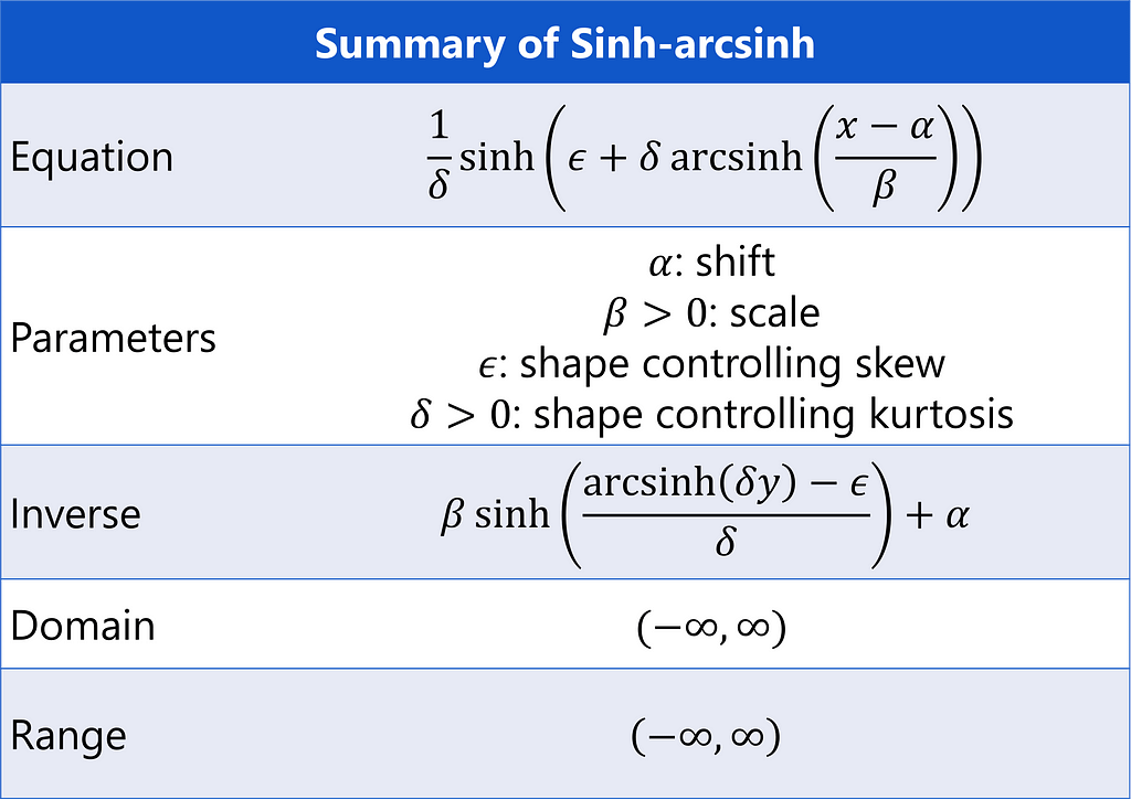
Proposed by Jones and Pewsey³, the sinh-arcsinh transformation is

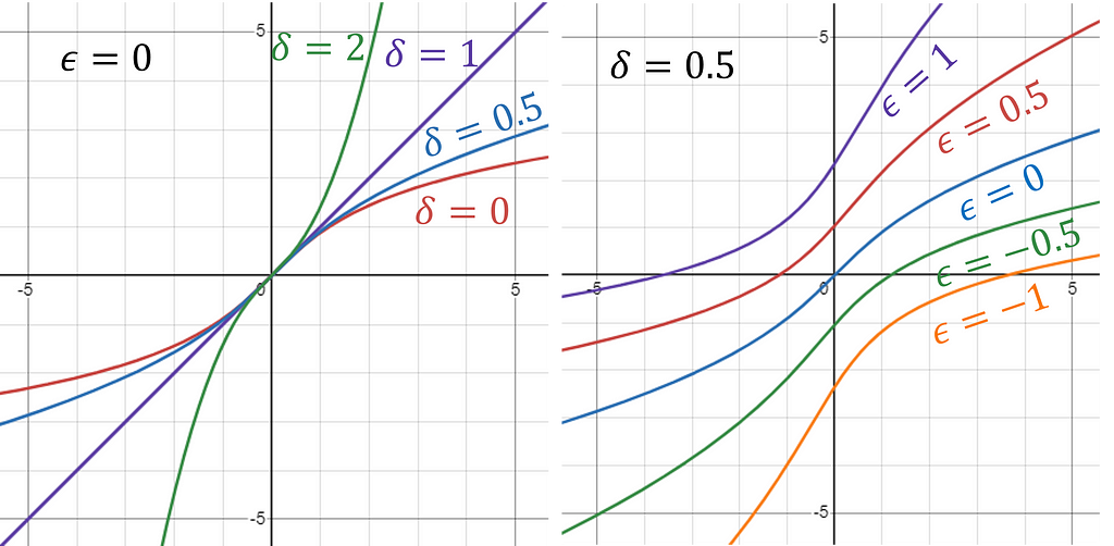
Parameter ε adjusts the skew of the data and δ adjusts the kurtosis³, allowing the transformation to take on many forms. For example, the identity transformation f(x) = x is a special case of sinh-arcsinh when ε = 0 and δ = 1. Arcsinh is a limiting case for ε = 0 and δ approaching zero, as can be seen using L’Hôpital’s rule again.

Scale Still Matters

Just like with arcsinh, there are meaningful differences in the results of the sinh-arcsinh transformation based on how your input data is shifted or scaled, meaning there are not two, but four parameters that can be chosen.

Parameter Estimation

We’ve seen how data transformations can make the tails of your data more Gaussian. Now, let’s take it to the next level by picking the parameters that maximize the normal log likelihood.

Let T(x) be my transformation, and let N(x | μ, σ) be the probability density function for a normal distribution with mean μ and standard deviation σ. Assuming independence, the likelihood of the entire dataset X is

where I’ve made use of the Jacobian of the transformation. The log likelihood is

where I can drop the absolute value signs because the derivative of the transformation is always positive.

Gradient Descent

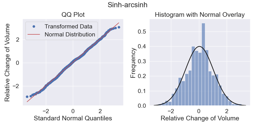
I estimate my parameters with gradient descent, setting the loss function to the negative mean log likelihood. Tensorflow’s GradientTape automatically calculates the partial derivatives with respect to the four parameters of sinh-arcsinh as well as μ and σ from the normal probability density function. Parameters β, δ, and σ are represented in log form to ensure they stay positive. You may want to try a few initializations of the variables in case the algorithm gets stuck at a local minimum. I also recommend normalizing your inputs to mean zero and standard deviation one before running the script for the best performance.

import tensorflow as tf
import numpy as np

@tf.function
def log_prob(x, params):
    # extract parameters
    alpha, log_beta = params[0], params[1]  # rescaling params
    beta = tf.math.exp(log_beta)
    epsilon, log_delta = params[2], params[3]  # transformation params
    delta = tf.math.exp(log_delta)
    mu, log_sigma = params[4], params[5]  # normal dist params
    sigma = tf.math.exp(log_sigma)
    # rescale
    x_scaled = (x - alpha)/beta
    # transformation
    sinh_arg = epsilon + delta * tf.math.asinh(x_scaled)
    x_transformed = (1/delta) * tf.math.sinh(sinh_arg)
    # log jacobian of transformation
    d_sinh = tf.math.log(tf.math.cosh(sinh_arg))
    d_arcsinh = - 0.5*tf.math.log(x_scaled**2 + 1)
    d_rescaling = - log_beta
    jacobian =  d_sinh + d_arcsinh + d_rescaling  # chain rule
    # normal likelihood
    z = (x_transformed - mu)/sigma  # standardized
    normal_prob = -0.5*tf.math.log(2*np.pi) - log_sigma -0.5*z**2
    return normal_prob + jacobian

# Learning rate and number of epochs
learning_rate = 0.1
epochs = 1000

# Initialize variables
tf.random.set_seed(892)
params = tf.Variable(tf.random.normal(shape=(6,), mean=0.0, stddev=1.0), dtype=tf.float32)

# Use the Adam optimizer
optimizer = tf.optimizers.Adam(learning_rate=learning_rate)

# Perform gradient descent
for epoch in range(epochs):
    with tf.GradientTape() as tape:
        loss = - tf.reduce_mean(log_prob(x_tf, params))

    # Compute gradients
    gradients = tape.gradient(loss, [params])

    # Apply gradients to variables
    optimizer.apply_gradients(zip(gradients, [params]))

    if (epoch % 100) == 0:
        print(-loss.numpy())

print(f"Optimal vals: {params}")

This optimized approach resulted in a distribution very close to Gaussian — not only the tails, but the mid-section too!

Conclusion

Log and Box-Cox are powerful transformations when working with positive data, but merely shifting these transformations to include negative values has severe limitations. The arcsinh transformation is much better at handling extreme positive and negative values simultaneously.

If you are willing to increase the complexity, the sinh-arcsinh transformation is a more powerful function that generalizes arcsinh. When normality is very important, its parameters can also be derived using gradient descent to match a Gaussian distribution.

Arcsinh doesn’t get much attention, but it’s an essential transformation that should be a part of every data engineer’s tool kit.

If you’ve found these transformation techniques useful or have any questions about applying them to your own datasets, please share your thoughts and experiences in the comments below.

Unless otherwise noted, all images are by the author.

Note from Towards Data Science’s editors: While we allow independent authors to publish articles in accordance with our rules and guidelines, we do not endorse each author’s contribution. You should not rely on an author’s works without seeking professional advice. See our Reader Terms for details.

[1] Jabbar, H. K., & Khan, R. Z. (2014). Methods to avoid over-fitting and under-fitting in supervised machine learning (Comparative study).

[2] CNNpred: CNN-based stock market prediction using a diverse set of variables. (2019). UCI Machine Learning Repository.

[3] Jones, M & Pewsey, Arthur. (2009). Sinh-arcsinh distributions: a broad family giving rise to powerful tests of normality and symmetry. Biometrika.

Transform Data with Hyperbolic Sine was originally published in Towards Data Science on Medium, where people are continuing the conversation by highlighting and responding to this story.