Robust One-Hot Encoding

Production grade one-hot encoding techniques in Python and R

Have you faced a crash in your machine learning production environments?

It’s not fun, and especially when it comes to issues that could be avoided. One issue that frequently causes problems is one-hot encoding of data. Drawing from my own experience, I’ve learned that many of these issues can largely be avoided by following a few best practices related to one-hot encoding. In this article I will briefly introduce the topic with a few simple examples and share some best practices to ensure stability of your machine learning models.

One-hot encoding

What is one-hot encoding?

One-hot encoding is the practice of turning a factor variable that is stored in a column into dummy variables stored over multiple columns and represented as 0s and 1s. A simple example illustrates the concept.

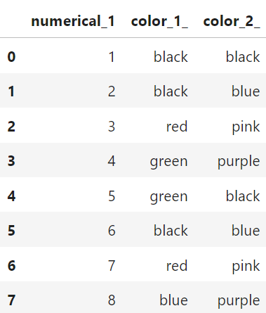
Consider for example this dataset with some numbers and some columns for colours:

import pandas as pd

# Creating the training_data DataFrame in Python
training_data = pd.DataFrame({
    'numerical_1': [1, 2, 3, 4, 5, 6, 7, 8],
    'color_1_': ['black', 'black', 'red', 'green', 
                'green', 'black', 'red', 'blue'],
    'color_2_': ['black', 'blue', 'pink', 'purple', 
                'black', 'blue', 'pink', 'purple']
})

Or more visually:

The column color_1_could also be represented like in the table below:

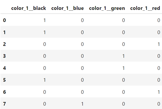
Changing color_1_ from a one-column compact representation of a categorical variable into a multi-column binary representation is what we call one-hot encoding.

Why do we use it?

There are multiple reasons to use one-hot encoding. They could be related to avoiding implicit ordering, improving model performance, or just making the data compatible with various algorithms.

For example, when you encode a categorical variable like colour, into a numerical structure, (e.g. 1 for black, 2 for green, 3 for red) without converting it to dummy variables, a model could mistakenly misinterpret the data to imply an order ( black < green < red) when no such order exists.

Also, when training neural nets, it is best practice to normalize the data before sending it into the neural net, and with categorical variables, one-hot encoding can be a good method. Other linear models, like logistic and linear regression assume linear relationships and numerical inputs so for this class of models, one-hot encoding can be a good idea as well.

In addition, the process of doing one-hot encoding forces us to ensure we don’t feed unseen factor levels into our machine learning models.

Ultimately, one-hot encoding makes it easier for the machine learning models to interpret the data and thus make better predictions.

The main reasons why one-hot encoding fails

The way we build traditional machine learning models is to first train the models on a “training dataset” — typically a dataset of historic values — and then later we generate predictions on a new dataset, the “inference dataset.” If the columns of the training dataset and the inference dataset don’t match, your machine learning algorithm will usually fail. This is primarily due to either missing or new factor levels in the inference dataset.

The first problem: Missing factors

For the following examples, assume that you used the dataset above to train your machine learning model. You one-hot encoded the dataset into dummy variables, and your fully transformed training data looks like below:

Now, let’s introduce the inference dataset, this is what you would use for making predictions. Let’s say it is given like below:

# Creating the inference_data DataFrame in Python
inference_data = pd.DataFrame({
    'numerical_1': [11, 12, 13, 14, 15, 16, 17, 18],
    'color_1_': ['black', 'blue', 'black', 'green', 
                'green', 'black', 'black', 'blue'],
    'color_2_': ['orange', 'orange', 'black', 'orange', 
                'black', 'orange', 'orange', 'orange']
})

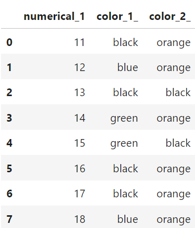
Using a naive one-hot encoding strategy like we used above (pd.get_dummies)

# Converting categorical columns in inference_data to 
# Dummy variables with integers
inference_data_dummies = pd.get_dummies(inference_data, 
  columns=['color_1_', 'color_2_']).astype(int)

This would transform your inference dataset in the same way, and you obtain the dataset below:

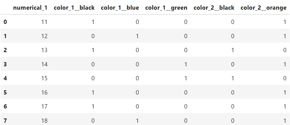
Do you notice the problems? The first problem is that the inference dataset is missing the columns:

missing_colmns =['color_1__red', 'color_2__pink', 
  'color_2__blue', 'color_2__purple']

If you ran this in a model trained with the “training dataset” it would usually crash.

The second problem: New factors

The other problem that can occur with one-hot encoding is if your inference dataset includes new and unseen factors. Consider again the same datasets as above. If you examine closely, you see that the inference dataset now has a new column: color_2__orange.

This is the opposite problem as previously, and our inference dataset contains new columns which our training dataset didn’t have. This is actually a common occurrence and can happen if one of your factor variables had changes. For example, if the colours above represent colours of a car, and a car producer suddenly started making orange cars, then this data might not be available in the training data, but could nonetheless show up in the inference data. In this case you need a robust way of dealing with the issue.

One could argue, well why don’t you list all the columns in the transformed training dataset as columns that would be needed for your inference dataset? The problem here is that you often don’t know what factor levels are in the training data upfront.

For example, new levels could be introduced regularly, which could make it difficult to maintain. On top of that comes the process of then matching your inference dataset with the training data, so you would need to check all actual transformed column names that went into the training algorithm, and then match them with the transformed inference dataset. If any columns were missing you would need to insert new columns with 0 values and if you had extra columns, like the color_2__orange columns above, those would need to be deleted. This is a rather cumbersome way of solving the issue, and thankfully there are better options available.

The solution

The solution to this problem is rather straightforward, however many of the packages and libraries that attempt to streamline the process of creating prediction models fail to implement it well. The key lies in having a function or class that is first fitted on the training data, and then use that same instance of the function or class to transform both the training dataset and the inference dataset. Below we explore how this is done using both Python and R.

In Python

Python is arguably one the best programming language to use for machine learning, largely due to its extensive network of developers and mature package libraries, and its ease of use, which promotes rapid development.

Regarding the issues related to one-hot encoding we described above, they can be mitigated by using the widely available and tested scikit-learn library, and more specifically the sklearn.preprocessing.OneHotEncoder class. So, let’s see how we can use that on our training and inference datasets to create a robust one-hot encoding.

from sklearn.preprocessing import OneHotEncoder

# Initialize the encoder
enc = OneHotEncoder(handle_unknown='ignore')

# Define columns to transform
trans_columns = ['color_1_', 'color_2_']

# Fit and transform the data
enc_data = enc.fit_transform(training_data[trans_columns])

# Get feature names
feature_names = enc.get_feature_names_out(trans_columns)

# Convert to DataFrame
enc_df = pd.DataFrame(enc_data.toarray(), 
                          columns=feature_names)

# Concatenate with the numerical data
final_df = pd.concat([training_data[['numerical_1']], 
                      enc_df], axis=1)

This produces a final DataFrameof transformed values as shown below:

If we break down the code above, we see that the first step is to initialize the an instance of the encoder class. We use the option handle_unknown=’ignore’ so that we avoid issues with unknow values for the columns when we use the encoder to transform on our inference dataset.

After that, we combine a fit and transform action into one step with the fit_transform method. And finally, we create a new data frame from the encoded data and concatenate it with the rest of the original dataset.

Now the task remains to use the encoder to transform our inference dataset.

# Transform inference data
inference_encoded = enc.transform(inference_data[trans_columns])

inference_feature_names = enc.get_feature_names_out(trans_columns)

inference_encoded_df = pd.DataFrame(inference_encoded.toarray(), 
                                    columns=inference_feature_names)

final_inference_df = pd.concat([inference_data[['numerical_1']], 
                                inference_encoded_df], axis=1)

Unlike earlier, when we used the naive pandas.get_dummies ,we now see that our new final_inference_df dataset has the same columns as our training dataset.

In addition to what we showed in the code above, the OneHotEncoder class from sklearn.preprocessing has a lot of other functionality that can be useful as well.

For example, it allows you set the min_frequency and max_categories options. As its name implies the min_frequency options allow you to specify the minimum frequency below which a category will be considered infrequent and then grouped together with other infrequent categories, or the max_categories option which limits the total number of categories. The latter can be especially useful if you don’t want to create too many columns in your training dataset.

For a full overview of the functionality, visit the documentation pages here:

sklearn.preprocessing.OneHotEncoder

In R

Several of my clients use R for running machine learning models in production — and it has a lot of great features. Before polars came out for Python, R’s data.table package was superior to what pandas could offer in terms of speed and efficiency. However, R doesn’t have access to the same type of production level packages as scikit-learn for python. (There are a few libraries, but they are not as mature as scikit-learn.) In addition, while some packages might have the required functionality, they require loads of other packages to run and can introduce dependency conflicts into your code. Consider running the line below in a docker container build with the r-base image:

RUN R -e "install.packages('recipes', dependencies=TRUE, repos='https://cran.rstudio.com/')"

It takes forever to install and takes up a lot of space on your container image. Our solution in this case — instead of using functions from a pre-built package like recipes — is to introduce our own simple function implemented using the data.table package:

library(data.table)

OneHotEncoder <- function() {
  # Local variables
  categories <- list()
  
  # Method to fit data and extract categories
  fit <- function(dt, columns) {
    for (column in columns) {
      categories[[column]] <<- unique(dt[[column]])
    }
  }
  
  # Method to turn columns into factors and 
  factorize <- function(dt) {
    for (column_name in names(categories)) {
        set(dt, j = column_name, 
        value = factor(dt[[column_name]], 
        levels = categories[[column_name]]))
    }
    return(dt)
  }
  
  # Method to transform columns in categories list to 
  # dummy variables
  transform <- function(dt) {
    dt = factorize(dt)
    # add row number for joins later
    dt[, rn := .I]
    for (col in names(categories)) {
      print(col)
      # Construct the formula dynamically
      formula_str <- paste("~", col, "- 1")
      formula_obj <- as.formula(formula_str)
      # Create a model model.matrix object
      mm = model.matrix(formula_obj, dt)
      mm_dt <- as.data.table(mm, keep.rownames = "rn")
      mm_dt[, rn := as.integer(rn)]
      
      # Perform a merge based on these row numbers
      dt <- merge(dt, mm_dt, by = "rn", all = TRUE)
      
       # remove the original column
      dt[, (col) := NULL]

      # set any new NAs to 0
      for (ncol in names(mm_dt)) {
        set(dt, which(is.na(dt[[ncol]])), ncol, 0)
      }
    }
    dt[, rn := NULL]
    return(dt)
  }

  # Method to get categories
  get_categories <- function() {
    return(categories)
  }
  
  # Return a list of methods
  list(
    get_categories = get_categories,
    fit = fit,
    transform = transform
  )
}

Let’s go through this function and see how it works on our training and inference datasets. (R is slightly different from Python and instead of using a class, we use a parent function instead, which works in a similar way.)

First, we need to create an instance of the function:

 encoder = OneHotEncoder()

Then, just like with the OneHotEncoder class from sklearn.preprocessing, we also have a fit function inside our OneHotEncoder. We use the fit function on the training data, supplying both the training dataset and the columns we want to one-hot encode.

# Columns to one-hot encode
fit_columns = c("color_1_", "color_2")
# Use the fit method
encoder$fit(dt=training_data, columns=fit_columns)

The fit function simply loops through all the columns we want to use to for training and finds all the unique values each of the columns contain. This list of columns and their potential values is then used in the transform function. We now have a instance of a fitted one-hot encoder function and we can save it for later use using a R .RDS file.

saveRDS(encoder, "~/my_encoder.RDS")

To generate the one-hot encoded dataset we need for training, we run the transform function on the training data:

transformed_training_data = encoder$transform(training_data)

The transform function is a little bit more complicated than the fit function, and the first thing it does is to convert the supplied columns into factors — using the original unique values of the columns as factor levels. Then, we loop through each of the predictor columns and create model.matrix objects of the data. These are then added back to the original dataset and the original factor column is removed. We also make sure to set any of the missing values to 0.

We now get the exact same dataset as before:

And finally, when we need to one-hot encode our inference dataset, we then run the same instance of the encoder function on that dataset:

transformed_inference_data = encoder$transform(inference_data)

This process ensures we have the same columns in our transformed_inference_data as we do in our transformed_training_data.

Further considerations

Before we conclude there are a few extra considerations to mention. As with many other things in machine learning there isn’t always an easy answer as to when and how to use a specific technique. Even though it clearly mitigates some issues, new problems can also arise when doing one-hot encoding. Most commonly, these are related to how to deal with high cardinality categorical variables and how to deal with memory issues because of increasing the table size.

In addition, there are alternative coding techniques such as label encoding, embeddings, or target encodings which sometimes could be preferable to one-hot encoding.

Each of these topics is rich enough to warrant a dedicated article, so we will leave those for the interested reader to explore further.

Conclusion

We have shown how naive use of one-hot encoding techniques can lead to mistakes and problems with inference data, and we have also seen how to mitigate and resolve those issues using both Python and R. If left unresolved, poor management of one-hot encoding can potentially lead to crashes and problems with your inference, so it is strongly recommended to use more robust techniques—like either sklearn’s OneHotEncoder or the R function we developed.

Thanks for reading!

All the code presented and used in the article can be found in the following Github repo: https://github.com/hcekne/robust_one_hot_encoding

If you enjoyed reading this article and would like to access more content from me please feel free to connect with me on LinkedIn at https://www.linkedin.com/in/hans-christian-ekne-1760a259/ or visit my webpage at https://www.ekneconsulting.com/ to explore some of the services I offer. Don’t hesitate to reach out via email at [email protected]

Robust One-Hot Encoding was originally published in Towards Data Science on Medium, where people are continuing the conversation by highlighting and responding to this story.