The Math Behind “The Curse of Dimensionality”

Dive into the “Curse of Dimensionality” concept and understand the math behind all the surprising phenomena that arise in high dimensions.

In the realm of machine learning, handling high-dimensional vectors is not just common; it’s essential. This is illustrated by the architecture of popular models like Transformers. For instance, BERT uses 768-dimensional vectors to encode the tokens of the input sequences it processes and to better capture complex patterns in the data. Given that our brain struggles to visualize anything beyond 3 dimensions, the use of 768-dimensional vectors is quite mind-blowing!

While some Machine and Deep Learning models excel in these high-dimensional scenarios, they also present many challenges. In this article, we will explore the concept of the “curse of dimensionality”, explain some interesting phenomena associated with it, delve into the mathematics behind these phenomena, and discuss their general implications for your Machine Learning models.

Note that detailed mathematical proofs related to this article are available on my website as a supplementary extension to this article.

What is the curse of dimensionality?

People often assume that geometric concepts familiar in three dimensions behave similarly in higher-dimensional spaces. This is not the case. As dimension increases, many interesting and counterintuitive phenomena arise. The “Curse of Dimensionality” is a term invented by Richard Bellman (famous mathematician) that refers to all these surprising effects.

What is so special about high-dimension is how the “volume” of the space (we’ll explore that in more detail soon) is growing exponentially. Take a graduated line (in one dimension) from 1 to 10. There are 10 integers on this line. Extend that in 2 dimensions: it is now a square with 10 × 10 = 100 points with integer coordinates. Now consider “only” 80 dimensions: you would already have 10⁸⁰ points which is the number of atoms in the universe.

In other words, as the dimension increases, the volume of the space grows exponentially, resulting in data becoming increasingly sparse.

High-dimensional spaces are “empty”

Consider this other example. We want to calculate the farthest distance between two points in a unit hypercube (where each side has a length of 1):

• In 1 dimension (the hypercube is a line segment from 0 to 1), the maximum distance is simply 1.
• In 2 dimensions (the hypercube forms a square), the maximum distance is the distance between the opposite corners [0,0] and [1,1], which is √2, calculated using the Pythagorean theorem.
• Extending this concept to n dimensions, the distance between the points at [0,0,…,0] and [1,1,…,1] is √n. This formula arises because each additional dimension adds a square of 1 to the sum under the square root (again by the Pythagorean theorem).

Interestingly, as the number of dimensions n increases, the largest distance within the hypercube grows at an O(√n) rate. This phenomenon illustrates a diminishing returns effect, where increases in dimensional space lead to proportionally smaller gains in spatial distance. More details on this effect and its implications will be explored in the following sections of this article.

The notion of distance in high dimensions

Let’s dive deeper into the notion of distances we started exploring in the previous section.

We had our first glimpse of how high-dimensional spaces render the notion of distance almost meaningless. But what does this really mean, and can we mathematically visualize this phenomenon?

Let’s consider an experiment, using the same n-dimensional unit hypercube we defined before. First, we generate a dataset by randomly sampling many points in this cube: we effectively simulate a multivariate uniform distribution. Then, we sample another point (a “query” point) from that distribution and observe the distance from its nearest and farthest neighbor in our dataset.

Here is the corresponding Python code.

def generate_data(dimension, num_points):
    ''' Generate random data points within [0, 1] for each coordinate in the given dimension '''
    data = np.random.rand(num_points, dimension)
    return data


def neighbors(data, query_point):
    ''' Returns the nearest and farthest point in data from query_point '''
    nearest_distance = float('inf')
    farthest_distance = 0
    for point in data:
        distance = np.linalg.norm(point - query_point)
        if distance < nearest_distance:
            nearest_distance = distance
        if distance > farthest_distance:
            farthest_distance = distance
    return nearest_distance, farthest_distance

We can also plot these distances:

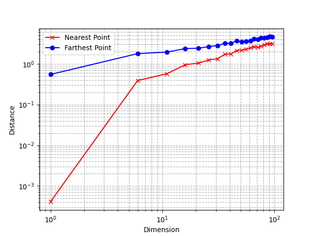
Using a log scale, we observe that the relative difference between the distance to the nearest and farthest neighbor tends to decrease as the dimension increases.

This is a very unintuitive behavior: as explained in the previous section, points are very sparse from each other because of the exponentially increasing volume of the space, but at the same time, the relative distances between points become smaller.

The notion of nearest neighbors vanishes

This means that the very concept of distance becomes less relevant and less discriminative as the dimension of the space increases. As you can imagine, it poses problems for Machine Learning algorithms that solely rely on distances such as kNN.

The maths: the n-ball

We will now talk about some other interesting phenomena. For this, we’ll need the n-ball. A n-ball is the generalization of a ball in n dimensions. The n-ball of radius R is the collection of points at a distance at most R from the center of the space 0.

Let’s consider a radius of 1. The 1-ball is the segment [-1, 1]. The 2-ball is the disk delimited by the unit circle, whose equation is x² + y² ≤ 1. The 3-ball (what we normally call a “ball”) has the equation x² + y² + z² ≤ 1. As you understand, we can extend that definition to any dimension:

The question now is: what is the volume of this ball? This is not an easy question and requires quite a lot of maths, which I won’t detail here. However, you can find all the details on my website, in my post about the volume of the n-ball.

After a lot of fun (integral calculus), you can prove that the volume of the n-ball can be expressed as follows, where Γ denotes the Gamma function.

For example, with R = 1 and n = 2, the volume is πR², because Γ(2) = 1. This is indeed the “volume” of the 2-ball (also called the “area” of a circle in this case).

However, beyond being an interesting mathematical challenge, the volume of the n-ball also has some very surprising properties.

As the dimension n increases, the volume of the n-ball converges to 0.

This is true for every radius, but let’s visualize this phenomenon with a few values of R.

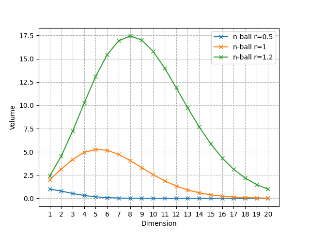
As you can see, it only converges to 0, but it starts by increasing and then decreases to 0. For R = 1, the ball with the largest volume is the 5-ball, and the value of n that reaches the maximum shifts to the right as R increases.

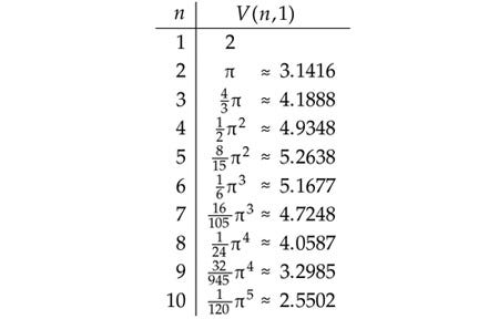
Here are the first values of the volume of the unit n-ball, up to n = 10.

The volume of a high-dimensional unit ball is concentrated near its surface.

For small dimensions, the volume of a ball looks quite “homogeneous”: this is not the case in high dimensions.

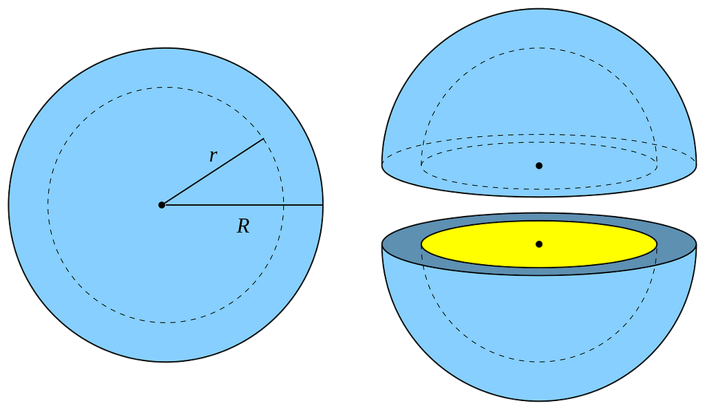
Let’s consider an n-ball with radius R and another with radius R-dR where dR is very small. The portion of the n-ball between these 2 balls is called a “shell” and corresponds to the portion of the ball near its surface(see the visualization above in 3D). We can compute the ratio of the volume of the entire ball and the volume of this thin shell only.

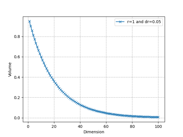
As we can see, it converges very quickly to 0: almost all the volume is near the surface in high dimensional spaces. For instance, for R = 1, dR = 0.05, and n = 50, about 92.3% of the volume is concentrated in the thin shell. This shows that in higher dimensions, the volume is in “corners”. This is again related to the distortion of the concept of distance we have seen earlier.

Note that the volume of the unit hypercube is 2ⁿ. The unit sphere is basically “empty” in very high dimensions, while the unit hypercube, in contrast, gets exponentially more points. Again, this shows how the idea of a “nearest neighbor” of a point loses its effectiveness because there is almost no point within a distance R of a query point q when n is large.

Curse of dimensionality, overfitting, and Occam’s Razor

The curse of dimensionality is closely related to the overfitting principle. Because of the exponential growth of the volume of the space with the dimension, we need very large datasets to adequately capture and model high-dimensional patterns. Even worse: we need a number of samples that grows exponentially with the dimension to overcome this limitation. This scenario, characterized by many features yet relatively few data points, is particularly prone to overfitting.

Occam’s Razor suggests that simpler models are generally better than complex ones because they are less likely to overfit. This principle is particularly relevant in high-dimensional contexts (where the curse of dimensionality plays a role) because it encourages the reduction of model complexity.

Applying Occam’s Razor principle in high-dimensional scenarios can mean reducing the dimensionality of the problem itself (via methods like PCA, feature selection, etc.), thereby mitigating some effects of the curse of dimensionality. Simplifying the model’s structure or the feature space helps in managing the sparse data distribution and in making distance metrics more meaningful again. For instance, dimensionality reduction is a very common preliminary step before applying the kNN algorithm. More recent methods, such as ANNs (Approximate Nearest Neighbors) also emerge as a way to deal with high-dimensional scenarios.

Blessing of dimensionality?

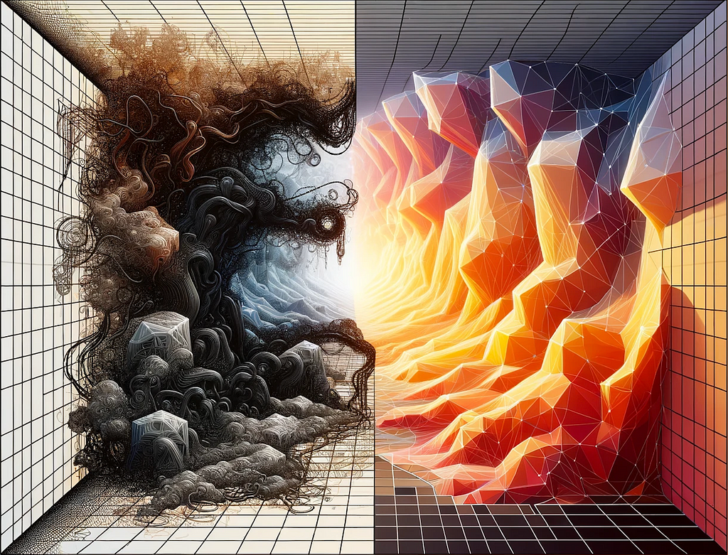
While we’ve outlined the challenges of high-dimensional settings in machine learning, there are also some advantages!

• High dimensions can enhance linear separability, making techniques like kernel methods more effective.
• Additionally, deep learning architectures are particularly adept at navigating and extracting complex patterns from high-dimensional spaces.

As always with Machine Learning, this is a trade-off: leveraging these advantages involves balancing the increased computational demands with potential gains in model performance.

Conclusion

Hopefully, this gives you an idea of how “weird” geometry can be in high-dimension and the many challenges it poses for machine learning model development. We saw how, in high-dimensional spaces, data is very sparse but also tends to be concentrated in the corners, and distances lose their usefulness. For a deeper dive into the n-ball and mathematical proofs, I encourage you to visit the extended of this article on my website.

While the “curse of dimensionality” outlines significant limitations in high-dimensional spaces, it’s exciting to see how modern deep learning models are increasingly adept at navigating these complexities. Consider the embedding models or the latest LLMs, for example, which utilize very high-dimensional vectors to more effectively discern and model textual patterns.

Want to learn more about Transformers and how they transform your data under the hood? Check out my previous article:

Transformers: How Do They Transform Your Data?

References:

• [1] “Volume of an n-ball.” Wikipedia, https://en.wikipedia.org/wiki/Volume_of_an_n-ball
• [2] “Curse of Dimensionality.” Wikipedia, https://en.wikipedia.org/wiki/Curse_of_dimensionality#Blessing_of_dimensionality
• [3] Peterson, Ivars. “An Adventure in the Nth Dimension.” American Scientist, https://www.americanscientist.org/article/an-adventure-in-the-nth-dimension
• [4] Zhang, Yuxi. “Curse of Dimensionality.” Geek Culture on Medium, July 2021, https://medium.com/geekculture/curse-of-dimensionality-e97ba916cb8f
• [5] “Approximate Nearest Neighbors (ANN).” Activeloop, https://www.activeloop.ai/resources/glossary/approximate-nearest-neighbors-ann/

The Math Behind “The Curse of Dimensionality” was originally published in Towards Data Science on Medium, where people are continuing the conversation by highlighting and responding to this story.