Interpretable Latent Spaces Using Space-Filling Vector Quantization

A new unsupervised method that combines two concepts of vector quantization and space-filling curves to interpret the latent space of DNNs

This post is a short explanation of our novel unsupervised distribution modeling technique called space-filling vector quantization [1] published at Interspeech 2023 conference. For more details, please look at the paper under this link.

Deep generative models are well-known neural network-based architectures that learn a latent space whose samples can be mapped to sensible real-world data such as image, video, and speech. Such latent spaces act as a black-box and they are often difficult to interpret. In this post, we introduce our novel unsupervised distribution modeling technique that combines two concepts of space-filling curves and vector quantization (VQ) which is called Space-Filling Vector Quantization (SFVQ). SFVQ helps to make the latent space interpretable by capturing its underlying morphological structure. Important to note that SFVQ is a generic tool for modeling distributions and using it is not restricted to any specific neural network architecture nor any data type (e.g. image, video, speech and etc.). In this post, we demonstrate the application of SFVQ to interpret the latent space of a voice conversion model. To understand this post you don’t need to know about speech signals technically, because we explain everything in general (not technical). Before everything, let me explain what is the SFVQ technique and how it works.

Space-Filling Vector Quantization (SFVQ)

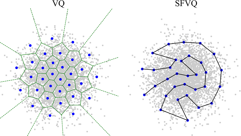
Vector quantization (VQ) is a data compression technique similar to k-means algorithm which can model any data distribution. The figure below shows a VQ applied on a Gaussian distribution. VQ clusters this distribution (gray points) using 32 codebook vectors (blue points) or clusters. Each voronoi cell (green lines) contains one codebook vector such that this codebook vector is the closest codebook vector (in terms of Euclidean distance) to all data points located in that voronoi cell. In other words, each codebook vector is the representative vector of all data points located in its corresponding voronoi cell. Therefore, applying VQ on this Gaussian distribution means to map each data point to its closest codebook vector, i.e. represent each data point with its closest codebook vector. For more information about VQ and its other variants you can check out this post.

Space-filling curve is a piece-wise continuous line generated with a recursive rule and if the recursion iterations are repeated infinitely, the curve gets bent until it completely fills a multi-dimensional space. The following figure illustrates the Hilbert curve [2] which is a well-known type of space-filling curves in which the corner points are defined using a specific mathematical formulation at each recursion iteration.

Getting intuition from space-filling curves, we can thus think of vector quantization (VQ) as mapping input data points on a space-filling curve (rather than only mapping data points exclusively on codebook vectors as what we do in normal VQ). Therefore, we incorporate vector quantization into space-filling curves, such that our proposed space-filling vector quantizer (SFVQ) models a D-dimensional data distribution by continuous piece-wise linear curves whose corner points are vector quantization codebook vectors. The following figure illustrates VQ and SFVQ applied on a Gaussian distribution.

For technical details on how to train SFVQ and how to map data points on SFVQ’s curve, please see section 2 in our paper [1].

Note that when we train a normal VQ on a distribution, the adjacent codebook vectors that exists inside the learned codebook matrix can refer to totally different contents. For example, the first codebook element could refer to a vowel phone and the second one could refer to a silent part of speech signal. However, when we train SFVQ on a distribution, the learned codebook vectors will be located in an arranged form such that adjacent elements in the codebook matrix (i.e. adjacent codebook indices) will refer to similar contents in the distribution. We can use this property of SFVQ to interpret and explore the latent spaces in Deep Neural Networks (DNNs). As a typical example, in the following we will explain how we used our SFVQ method to interpret the latent space of a voice conversion model [3].

Voice Conversion

The following figure shows a voice conversion model [3] based on vector quantized variational autoencoder (VQ-VAE) [4] architecture. According to this model, encoder takes the speech signal of speaker A as the input and passes the output into vector quantization (VQ) block to extracts the phonetic information (phones) out of this speech signal. Then, these phonetic information together with the identity of speaker B goes into the decoder which outputs the converted speech signal. The converted speech would contain the phonetic information (context) of speaker A with the identity of speaker B.

In this model, the VQ module acts as an information bottleneck that learns a discrete representation of speech that captures only phonetic content and discards the speaker-related information. In other words, VQ codebook vectors are expected to collect only the phone-related contents of the speech. Here, the representation of VQ output is considered the latent space of this model. Our objective is to replace the VQ module with our proposed SFVQ method to interpret the latent space. By interpretation we mean to figure out what phone each latent vector (codebook vector) corresponds to.

Interpreting the Latent Space using SFVQ

We evaluate the performance of our space-filling vector quantizer (SFVQ) on its ability to find the structure in the latent space (representing phonetic information) in the above voice conversion model. For our evaluations, we used the TIMIT dataset [5], since it contains phone-wise labeled data using the phone set from [6]. For our experiments, we use the following phonetic grouping:

• Plosives (Stops): {p, b, t, d, k, g, jh, ch}
• Fricatives: {f, v, th, dh, s, z, sh, zh, hh, hv}
• Nasals: {m, em, n, nx, ng, eng, en}
• Vowels: {iy, ih, ix, eh, ae, aa, ao, ah, ax, ax-h, uh, uw, ux}
• Semi-vowels (Approximants): {l, el, r, er, axr, w, y}
• Diphthongs: {ey, aw, ay, oy, ow}
• Silence: {h#}.

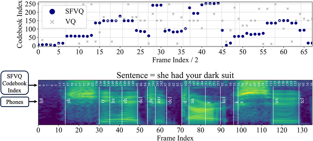
To analyze the performance of our proposed SFVQ, we pass the labeled TIMIT speech files through the trained encoder and SFVQ modules, respectively, and extract the codebook vector indices corresponding to all existing phones in the speech. In other words, we pass a speech signal with labeled phones and then compute the index of the learned SFVQ’s codebook vector which those phones are getting mapped to them. As explained above, we expect our SFVQ to map similar phonetic contents next to each other (index-wise in the learned codebook matrix). To examine this expectation, in the following figure we visualize the spectrogram of the sentence “she had your dark suit”, and its corresponding codebook vector indices for the ordinary vector quantizer (VQ) and our proposed SFVQ.

We observe that the indices of the ordinary VQ does not have any particular structure. However, when using our proposed SFVQ, there is a clear structure for the codebook vector indices. The indices for the speech frames containing fricative phones of {sh, s} within the words {she, suit} are uniformly distributed next to each other throughout the frames. In addition, silence frames containing phone {h#} and some other low energy frames containing {kcl, tcl: k, t closures} within the words {dark, suit} are uniformly located next to each other in the range [0–20]. Notice that the figure below remains sufficiently consistent for sentences with the same phonetic content, even across speakers with different genders, speech rhythms, and dialects.

The figure below demonstrates the histogram of SFVQ’s codebook indices for each phonetic group (explained above) for the whole TIMIT speech files. At first glance, we observe that consonants:{silence, plosives, fricatives, nasals} and vowels:{vowels, diphthongs, approximants} can be separated around index 125 (apart from the peak near index 20). We also observe that the most prominent peaks of different groups are separated in different parts of the histogram.

By having this visualization, we have a better understanding of the latent space and we can now distinguish which part of the latent space refers to what phonetic group. We can even go further in details and explore the latent space in terms of phone level. As an example for distribution of phones within a phonetic group, the figure below illustrates the histograms of all phones in fricatives group.

By observing the most prominent peak for each phone, we find out the peaks of similar phones are located next to each other. To elaborate, we listed similar phones and their corresponding peak index here as {f:51, v:50}, {th:78, dh:80}, {s:71, z:67, sh:65, zh:67}, {hh:46, hv:50}. Except {hh, hv} phones, fricatives are mainly located in the range [50–85]. Further structures can be readily identified from all provided figures by visual inspection.

These experiments demonstrate that our proposed SFVQ achieves a coherently structured and easily interpretable representation for latent codebook vectors, which represent phonetic information of the input speech. Accordingly, there is an obvious distinction of various phonetic groupings such as {consonants vs. vowels}, {fricatives vs. nasals vs. diphthongs vs. …}, and we can simply tell apart which phone each codebook vector represents. In addition, similar phones within a specific phonetic group are encoded next to each other in the latent codebook space. This is the main interpretability that we aimed to obtain from a black-box called latent space.

One advantage of SFVQ over other supervised approaches which tries to make the latent space interpretable is that SFVQ does not incur any human labeling and manual restrictions on the learned latent space. To make our method interpretable, it only requires the user to study the unsupervised learned latent space entirely once by observation. This observation needs much much less labeled data than what is necessary for supervised training of big models. Again we want to note that SFVQ is a generic tool for modeling distributions and using it is not restricted to any specific neural network architecture nor any data type (e.g. image, video, speech and etc.).

GitHub Repository

PyTorch implementation of our SFVQ technique is publicly available in GitHub using the following link:

GitHub – MHVali/Space-Filling-Vector-Quantizer

Acknowledgement

Special thanks to my doctoral program supervisor Prof. Tom Bäckström, who supported me and was the other contributor for this work.

References

[1] M.H. Vali, T. Bäckström, “Interpretable Latent Space Using Space-Filling Curves for Phonetic Analysis in Voice Conversion”, in Proceedings of Interspeech, 2023.

[2] H. Sagan, “Space-filling curves”, Springer Science & Business Media, 2012.

[3] B. Van Niekerk, L. Nortje, and H. Kamper, “Vector-quantized neural networks for acoustic unit discovery in the Zerospeech 2020 challenge”, in Proceedings of Interspeech, 2020.

[4] A. Van Den Oord, O. Vinyals, and K. Kavukcuoglu, “Neural Discrete Representation Learning,” in Proceedings of the 31st International Conference on Neural Information Processing Systems, 2017.

[5] J. S. Garofolo, L. F. Lamel, W. M. Fisher, J. G. Fiscus, D. S. Pallett, and N. L. Dahlgren, “The DARPA TIMIT Acoustic-Phonetic Continuous Speech Corpus CDROM”, Linguistic Data Consortium, 1993.

[6] C. Lopes and F. Perdigao, “Phoneme recognition on the TIMIT database”, in Speech Technologies. IntechOpen, 2011, ch. 14. [Online]. Available: https://doi.org/10.5772/17600

Interpretable Latent Spaces Using Space-Filling Vector Quantization was originally published in Towards Data Science on Medium, where people are continuing the conversation by highlighting and responding to this story.