Improving Generalization in Survival Models

Suggestions for estimating and enhancing predictive accuracy for the employee attrition case

Recently, I’ve come up with a particular issue when dealing with survival analysis: many models I fitted performed well in theory, with strong test metrics, but then failed to predict the true outcomes that were observed in practice. In this article, I want to discuss ways to better estimate the performance of our survival models, and a practical tip to help with extrapolation. Note: the main assumption here is that we count with several observations of our individuals over time (e.g., monthly observations for all the employees in a company).

The problem I was dealing with was the employee attrition case. I had information about several employees in a company, and I was interested in predicting which of them were most likely to leave in the future. If you want to explore the employee attrition topic further, make sure to check out this helpful article.

Traditional Approach

Many existing implementations on survival analysis start off with a dataset containing one observation per individual (patients in a health study, employees in the attrition case, clients in the client churn case, and so on). For these individuals we typically have two key variables: one signaling the event of interest (an employee quitting) and another measuring time (how long they’ve been with the company, up to either today or their departure). Together with these two variables, we then have explanatory variables with which we aim to predict the risk of each individual. These features can include the job role, age or compensation of the employee, for example.

Moving on, most implementations out there take a survival model (from simpler estimators such as Kaplan Meier to more complex ones like ensemble models or even neural networks), fit them over a train set and then evaluate over a test set. This train-test split is usually performed over the individual observations, generally making a stratified split.

In my case, I started with a dataset that followed several employees in a company monthly until December 2023 (in case the employee was still at the company), or until the month they left the company — the event date:

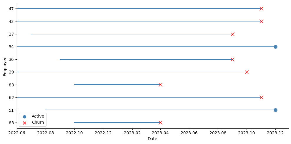
In order to adapt my data to the survival case, I took the last observation of each employee as shown in the picture above (the blue dots for active employees, and the red crosses for employees who left). At that point for each employee, I recorded whether the event had occurred at that date or not (if they were active or if they had left), their tenure in months at that time, and all their explanatory variables. I then performed a stratified train-test split over this data, like this:

import numpy as np
import pandas as pd
from sklearn.model_selection import train_test_split

# We load our dataset with several observations (record_date) per employee (employee_id)
# The event column indicates if the employee left on that given month (1) or if the employee was still active (0)
df = pd.read_csv(f'{FILE_NAME}.csv')

# Creating a label where positive events have tenure and negative events have negative tenure - required by Random Survival Forest
df_model['label'] = np.where(df_model['event'], df_model['tenure_in_months'], - df_model['tenure_in_months'])

df_train, df_test = train_test_split(df_model, test_size=0.2, stratify=df_model['event'], random_state=42)

After performing the split, I proceeded to fit a model. In this case, I chose to experiment with a Random Survival Forest using the scikit-survival library.

from sklearn.preprocessing import OrdinalEncoder
from sksurv.datasets import get_x_y
from sksurv.ensemble import RandomSurvivalForest

cat_features = [] # list of all the categorical features
features = [] # list of all the features (both categorical and numeric)

# Categorical Encoding
encoder = OrdinalEncoder(handle_unknown='use_encoded_value', unknown_value=-1)
encoder.fit(df_train[cat_features])

df_train[cat_features] = encoder.transform(df_train[cat_features])
df_test[cat_features] = encoder.transform(df_test[cat_features])

# X & y
X_train, y_train = get_x_y(df_train, attr_labels=['event','tenure_in_months'], pos_label=1)
X_test, y_test = get_x_y(df_test, attr_labels=['event','tenure_in_months'], pos_label=1)

# Fit the model
estimator = RandomSurvivalForest(random_state=RANDOM_STATE)
estimator.fit(X_train[features], y_train)

# Store predictions
y_pred = estimator.predict(X_test[features])

After a quick run using the default settings of the model, I was thrilled with the test metrics I saw. First of all, I was getting a concordance index above 0.90 in the test set. The concordance index is a measure of how well the model predicts the order of events: it reflects whether employees predicted to be at high risk were indeed the ones leaving the company first. An index of 1 corresponds to perfect prediction accuracy, while an index of 0.5 indicates a prediction no better than random chance.

I was particularly interested in seeing if the employees who left in the test set matched with the most risky employees according to the model. In the case of the Random Survival Forest, the model returns the risk scores of each observation. I took the percentage of employees who left the company in the test set, and used it to filter the most risky employees according to the model. The results were very solid, with the employees flagged with the most risk matching almost perfectly with the actual leavers, with an F1 score above 0.90 in the minority class.

from lifelines.utils import concordance_index
from sklearn.metrics import classification_report

# Concordance Index
ci_test = concordance_index(df_test['tenure_in_months'], -y_pred, df_test['event'])
print(f'Concordance index:{ci_test:0.5f}n')

# Match the most risky employees (according to the model) with the employees who left
q_test = 1 - df_test['event'].mean()

thr = np.quantile(y_pred, q_test)
risky_employees = (y_pred >= thr) * 1

print(classification_report(df_test['event'], risky_employees))

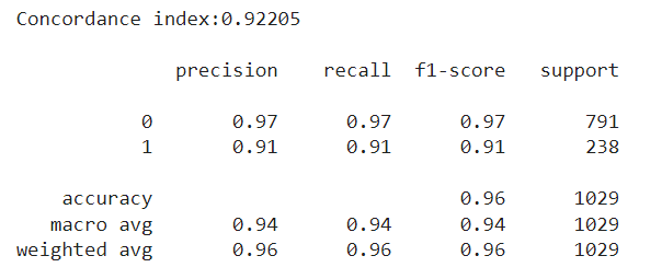
Getting +0.9 metrics on the first run should set off an alarm: was the model really able to predict whether an employee was going to stay or leave with such confidence? Imagine this: we submit our predictions saying which employees are most likely to leave. However, a couple months go by, and HR then reaches us worried, saying that the people who left during the last period, did not exactly match with our predictions, at least at the rate it was expected from our test metrics.

We have two main problems here: the first one is that our model isn’t extrapolating quite as well as we thought. The second one, and even worse, is that we weren’t able to measure this lack of performance. First, I’ll show a simple way we can estimate how well our model is truly extrapolating, and then I’ll talk about one potential reason it may be failing to do so, and how to mitigate it.

Estimating Generalization Capabilities

The key here is having access to panel data, that is, several records of our individuals over time, up until the time of event or the time the study ended (the date of our snapshot, in the case of employee attrition). Instead of discarding all this information and keeping only the last record of each employee, we could use it to create a test set that will better reflect how the model performs in the future. The idea is quite simple: suppose we have monthly records of our employees up until December 2023. We could move back, say, 6 months, and pretend we took the snapshot in June instead of December. Then, we would take the last observation for employees who left the company before June 2023 as positive events, and the June 2023 record of employees who survived beyond that date as negative events, even if we already know some of them eventually left afterwards. We are pretending we don’t know this yet.

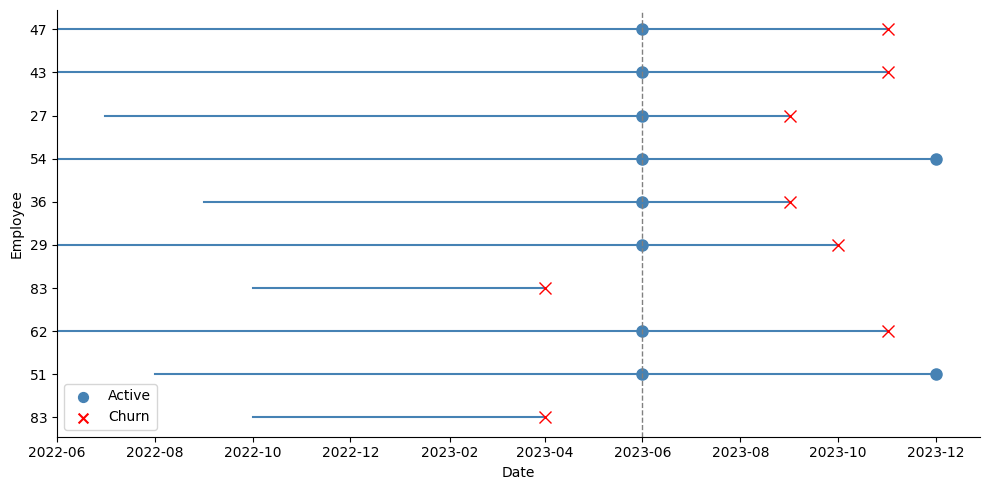
As the picture above shows, I take a snapshot in June, and all employees who were active at that time are taken as active. The test dataset takes all those active employees at June with their explanatory variables as they were on that date, and takes the latest tenure they achieved by December:

test_date = '2023-07-01'

# Selecting training data from records before the test date and taking the last observation per employee
df_train = df[df.record_date < test_date].reset_index(drop=True).copy()
df_train = df_train.groupby('employee_id').tail(1).reset_index(drop=True)
df_train['label'] = np.where(df_train['event'], df_train['tenure_in_months'], - df_train['tenure_in_months'])

# Preparing test data with records of active employees at the test date
df_test = df[(df.record_date == test_date) & (df['event']==0)].reset_index(drop=True).copy()
df_test = df_test.groupby('employee_id').tail(1).reset_index(drop=True)
df_test = df_test.drop(columns = ['tenure_in_months','event'])

# Fetching the last tenure and event status for employees in the test dataset
df_last_tenure = df[df.employee_id.isin(df_test.employee_id.unique())].reset_index(drop=True).copy()
df_last_tenure = df_last_tenure.groupby('employee_id').tail(1).reset_index(drop=True)

df_test = df_test.merge(df_last_tenure[['employee_id','tenure_in_months','event']], how='left')
df_test['label'] = np.where(df_test['event'], df_test['tenure_in_months'], - df_test['tenure_in_months'])

We fit our model again on this new train data, and once we finish we make our predictions for all employees who were active on June. We then compare these predictions to the actual outcome of July — December 2023 — this is our test set. If those employees we marked as having the most risk left during the semester, and those we marked as having the lowest risk didn’t leave, or left rather late in the period, then our model is extrapolating well. By shifting our analysis back in time and leaving the last period for evaluation, we can have a better understanding of how well our model is generalizing. Of course, we could take this one step further and perform some type of time-series cross validation. For example, we could iterate this process many times, each time moving 6 months back in time, and evaluating the model’s accuracy over several time frames.

After training our model once again, we now see a drastic decrease in performance. First of all, the concordance index is now around 0.5 — equivalent to that of a random predictor. Also, if we try to match the ‘n’ most risky employees according to the model with the ‘n’ employees who left in the test set, we see a very poor classification with a 0.15 F1 for the minority class:

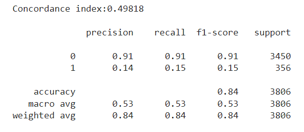
So clearly there is something wrong, but at least we are now able to detect it instead of being misled. The main takeaway here is that our model performs well with a traditional split, but doesn’t extrapolate when doing a time-based split. This is a clear sign that some time bias may be present. In short, time-dependent information is being leaked and our model is overfitting over it. This is common in cases like our employee attrition problem, when the dataset comes from a snapshot taken at some date.

Time Bias

The problem cuts down to this: all our positive observations (employees who left) belong to past dates, and all our negative observations (currently active employees) are all measured on the same date — today. If there is a single feature that reveals this to the model, then instead of predicting risk we will be predicting if an employee was recorded in December 2023 or before. This could be very subtle. For example, one feature we could be using is the engagement score of the employees. This feature could well show some seasonal patterns, and measuring it at the same time for active employees will surely introduce some bias in the model. Maybe in December, during the holiday season, this engagement score tends to decrease. The model will see a low score associated with all active employees, so it may learn to predict that whenever the engagement runs low, the churn risk also goes down, when in fact it should be the opposite!

By now, a simple yet quite effective solution for this problem should be clear: instead of taking the last observation for each active employee, we could just pick a random month from all their history within the company. This will strongly reduce the chances of the model picking on any temporal patterns that we do not want it to overfit on:

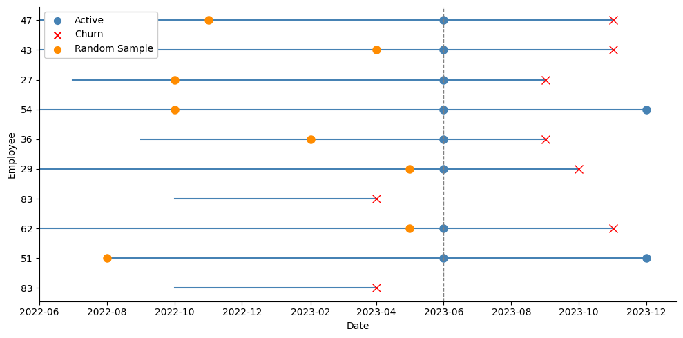
In the picture above we can see that we are now spanning a broader set of dates for the active employees. Instead of using their blue dots at June 2023, we take the random orange dots instead, and record their variables at the time, and the tenure they had so far in the company:

np.random.seed(0)

# Select training data before the test date
df_train = df[df.record_date < test_date].reset_index(drop=True).copy()

# Create an indicator for whether an employee eventually churns within the train set
df_train['indicator'] = df_train.groupby('employee_id').event.transform(max)

# Isolate records of employees who left, and store their last observation
churn = df_train[df_train.indicator==1].reset_index(drop=True).copy()
churn = churn.groupby('employee_id').tail(1).reset_index(drop=True)

# For employees who stayed, randomly pick one observation from their historic records
stay = df_train[df_train.indicator==0].reset_index(drop=True).copy()
stay = stay.groupby('employee_id').apply(lambda x: x.sample(1)).reset_index(drop=True)

# Combine churn and stay samples into the new training dataset
df_train = pd.concat([churn,stay], ignore_index=True).copy()
df_train['label'] = np.where(df_train['event'], df_train['tenure_in_months'], - df_train['tenure_in_months'])
del df_train['indicator']

# Prepare the test dataset similarly, using only the snapshot from the test date
df_test = df[(df.record_date == test_date) & (df.event==0)].reset_index(drop=True).copy()
df_test = df_test.groupby('employee_id').tail(1).reset_index(drop=True)
df_test = df_test.drop(columns = ['tenure_in_months','event'])

# Get the last known tenure and event status for employees in the test set
df_last_tenure = df[df.employee_id.isin(df_test.employee_id.unique())].reset_index(drop=True).copy()
df_last_tenure = df_last_tenure.groupby('employee_id').tail(1).reset_index(drop=True)

df_test = df_test.merge(df_last_tenure[['employee_id','tenure_in_months','event']], how='left')
df_test['label'] = np.where(df_test['event'], df_test['tenure_in_months'], - df_test['tenure_in_months'])

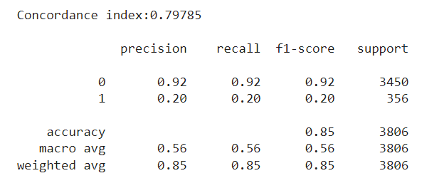
We then train our model once again, and evaluate it over the same test set we had before. We now see a concordance index of around 0.80. This isn’t the +0.90 we had earlier, but it definitely is a step up from the random-chance level of 0.5. Regarding our interest in classifying employees, we are still very far off the +0.9 F1 we had before, but we do see a slight increase compared to the previous approach, especially for the minority class.

Closing Remarks

To sum up, here are the main takeaways from our discussion:

• It’s important to pay attention to the dates the observations were recorded — there is a high chance some sort of time bias is present, especially if all the observations of one of the event classes share the same date
• If we have past observations for our individuals, we can better estimate the performance of our models by setting aside a time period for testing, instead of performing a traditional train-test split over the individual observations
• If there is a strong performance decrease between the traditional approach and the time-based test split, this could be a sign of time bias
• One simple way to mitigate this, at least in part, is to randomly choose observations for each individual, instead of taking their last record for each

I hope this walkthrough was useful. If you’ve been dealing with similar issues in survival analysis, I’d love to hear whether this approach works for you too. Thanks for reading!

Improving Generalization in Survival Models was originally published in Towards Data Science on Medium, where people are continuing the conversation by highlighting and responding to this story.