Exploring Location Data Using a Hexagon Grid

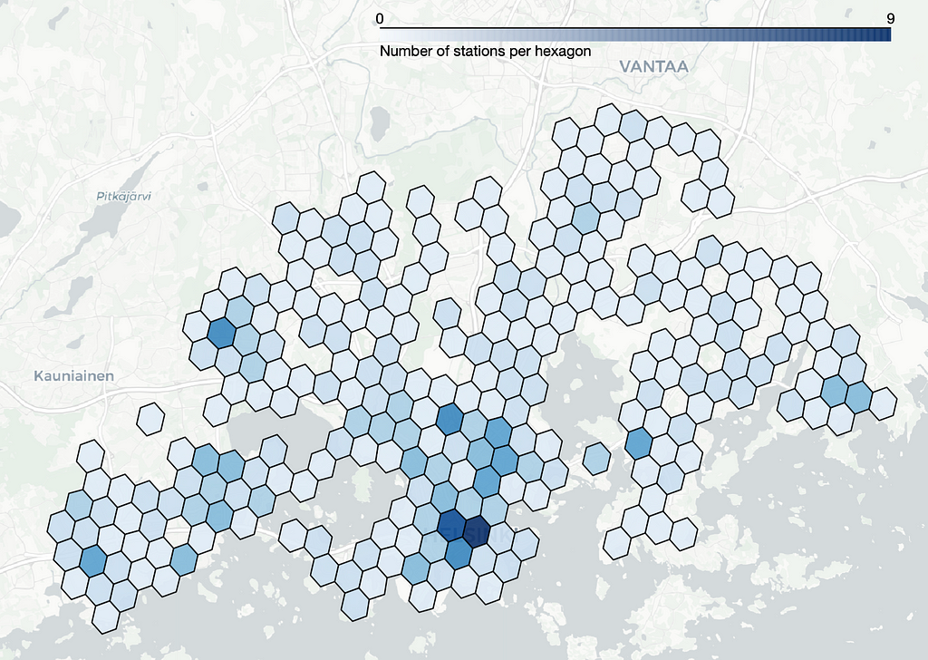
A comprehensive guide on how to use Uber’s H3 hexagon grid in data analysis

Uber’s global H3 hexagonal grid system can be used for two purposes: first, it is a user-friendly and practical tool for spatial data analysis. Second, it can be used to anonymize location data by aggregating geographic information to hexagonal regions such that no precise locations are disclosed. In this article, we use Helsinki city bike data to showcase how hexagons can help data scientists in their work.

Many services nowadays produce data that contains events that have occurred in a certain location. For example there’s a lot of different courier services that might want to understand where and when their services have been used, or teleoperator companies that want to know how big load their network must tolerate at certain times at different parts of their cover area. Also location data can be highly sensitive and reveal unnecessary exact information on users whereabouts. For example, openly available New York taxi data contains exact information on the pick-up and drop-off dates, times and locations of all taxi rides in New York. By using information from paparazzis on where and when celebrities have been seen getting in and out of the cabs, the tabloid magazines have used the taxi data to track celebs’ visits to bars and strip clubs (source).

For these reasons it is convenient to bucket location data points into larger groups. However, defining these location clusters is not entirely straightforward. Sometimes one can use countries, counties, cities or districts to group data points together but often there’s a need for finer regions. For this purpose Uber developed an open-sourced geospatial grid system called H3 that covers the entire Earth with repetitive tiling. The building block in the grid system is a hexagon and one can choose from 16 different hexagon sizes that vary from an area of a large country to an area of a small side table.

In this article, we will use Helsinki city bike data to demonstrate how one can utilise H3 hexagons to analyse spatial data. First, we provide an introduction to the H3 hexagon grid and its resolutions. Next, we delve into the main functionalities of the H3 library. Following that, we illustrate how a hexagon grid can enhance data analysis. Finally, we address some issues associated with hexagonal grids. All the notebooks used in this analysis can be found on this GitHub repository. All images in this article, unless otherwise noted, are by the author.

Uber’s H3 hexagon system — great for visualising, exploring and optimising spatial data

Every day and every minute, Uber receives multiple requests in their marketplace. Each event happens at a specific location, for example a rider asks for a ride in one location and a driver accepts the drive in a nearby location. Deriving information and insights from the data, for example setting dynamical pricing that is based on the demand, requires analyzing data across an entire city. But as cities are geographically very diverse, this analysis must happen in fine granularity. With the H3 hexagon grid system, each data point can be bucketed to one hexagon area or cell, and then one Uber can calculate supply and demand for surge pricing on each hexagon in all the cities where they have services. The hexagons come in different sizes so one must choose the resolution that best fits the purpose of the analysis.

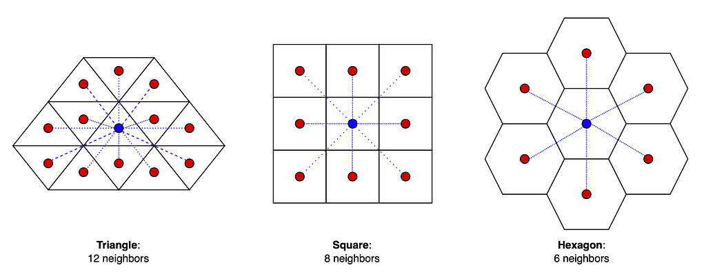
Technically one could build a global grid system using any kind of building block that facilitates a complete tiling throughout the 3D globe. For example one could use triangles (3 sides) or squares (4 sides) instead of hexagons (6 sides) to cover the whole Earth. However, using hexagons has many advantages. For example, the centerpoint of a triangle has three and a square has two different distances to its neighbors’ centerpoints whereas the centerpoint of a hexagon has equal distance to all of its neighbors’ which makes it a convenient system to approximate radiuses (see image below).

However, the world cannot be divided completely into hexagons so few pentagons (five sides) are needed as well (12 to be exact, on each resolution). The pentagons introduce discontinuities to the grid but often they are located far away from the land so it causes problems for mainly marine data analysis. Despite the presence of a few pentagons, the hexagon grid offers the advantage of providing building blocks that are relatively uniform in size on the 3D spherical surface. In case one wants to read more about the geometrics of a hexagon grid, here’s a good source for it. Note that defining the hexagon regions is highly arbitrary, and they do not follow any natural features such as lakes, rivers, mountains or country borders.

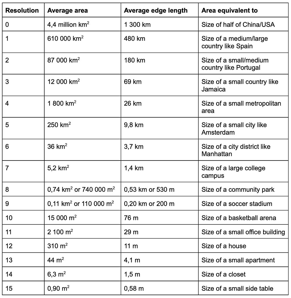
The H3 library is open source, available on GitHub and written in C. It has bindings available on multiple languages, for example on Python, C, Java and Javascript. H3 comes with a hierarchical indexing system which makes it very efficient. One can examine the hexagons further using an online H3 hexagon data viewer. The table below summarizes the properties of the 16 different resolutions that H3 provides.

Next, we will introduce some of the most important functionalities of the H3 library.

H3 library and its main functions

In this article we will use the H3 hexagon system to cluster location data into hexagons. The documentation of H3 library can be found here. There are two main versions of this library, versions 3 and 4, and in our notebooks we will use version 3.7.6. Note that there are significant differences in function names between version 3.x and 4.x as listed in here.

H3 Python package is easy to install for example with pip:

pip install h3

If you want to specify which version you want to use, add there the version number, for example h3==3.7.6. Then import H3 to your Python notebook with

import h3

Next, we will introduce some of the most important functions of the H3 library.

Hexagon index

H3 uses a hierarchical indexing system, which transforms latitude and longitude pairs to a 64-bit H3 index that identifies each grid cell. With given coordinates (latitude and longitude) and with selected resolution, we get the hexagon index:

# Version 3.X:
hexagon_index = h3.geo_to_h3(lat, lng, resolution)

# Version 4.X:
hexagon_index = h3.latlng_to_cell(lat, lng, resolution)

For example

h3.geo_to_h3(60.169833, 24.938163, 6)

returns index ‘861126d37ffffff’. If you want, you can use an online H3 hexagon data viewer to check where this hexagon is located.

So when we know the precise coordinates for a data point, we can determine its hexagon index at various resolutions and associate it with hexagons of different sizes.

Hexagon boundaries

To use hexagons in our plots, we must determine the hexagon boundaries from the hexagon index. Note that coordinates in some systems are presented as (lng, lat), while in others, they follow the format (lat, lng). The geo_json=True/False option allows you to swap these coordinates.

# Version 3.X:
boundary = h3.h3_to_geo_boundary(hexagon_index, geo_json = False)

# Version 4.X:
boundary = h3.cell_to_boundary(hexagon_index, geo_json = False)

For example

h3.h3_to_geo_boundary('861126d37ffffff', geo_json = False)

# Returns:
((60.15652369744344, 24.856525761155346),
 (60.13498207546084, 24.895664284494664),
 (60.14431977678549, 24.948769321085937),
 (60.175221029708474, 24.962796993345798),
 (60.19677983831024, 24.92362795620145),
 (60.187420192445906, 24.870461733016352))

These six coordinate pairs correspond to the starting and ending points of the hexagon edges.

Neighboring hexagons

Sometimes we need to identify the neighbors of a specific hexagon, or “kring” around the hexagon. With k=0 the function returns the origin index, with k=1 it returns the origin index and its all neighboring indices, and with k=2 it returns the origin index, its neighboring and next-to-neighboring indices, and so forth.

# Version 3.X:
kring = h3.k_ring(hexagon_index, k)

# Version 4.X:
kring = h3.grid_disk(hexagon_index, k)

Also there’s a function that can be used to calculate the grid distance between two cells:

# Version 3.X:
kring = h3.h3_distance(hexagon_index_a, hexagon_index_a)

# Version 4.X:
kring = h3.grid_distance(hexagon_index_a, hexagon_index_a)

We can use these functions in the following way:

# Nearest neighbours of the hexagon:
h3.k_ring('861126d37ffffff', 1)

# Returns:
{'86089969fffffff',
 '86089ba4fffffff',
 '86089ba6fffffff',
 '861126d07ffffff',
 '861126d17ffffff',
 '861126d27ffffff',
 '861126d37ffffff'}

# Distance between two hexagons:
h3.h3_distance('861126d37ffffff', '86089ba4fffffff')

# Returns
1

Plotting the hexagons

There are multiple ways on how to plot hexagons on a map but some of them are quite stiff, time consuming to use and not well-documented. For simplicity, we are mainly using matplotlib for visualizations but we also experiment and take screenshots of visualizations with folium maps. More details on these plotting methods can be found from the GitHub repository.

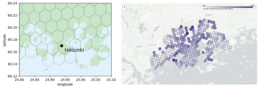
On the left in the above figure we use matplotlib for plotting the hexagons. We utilize the GADM library to fetch the multipolygon representing the Helsinki region and plot it with green color. We use blue in the background to represent bodies of water. Additionally, we include a marker denoting the Helsinki city center on the map. The hexagons are easily rendered using the plot_polygon function from the shapely library and data points can be added to the plot by using scatterplot. This makes the plotting very easy and quick.

We also experimented with other plotting methods, such as using folium maps that allows us to create an interactive HTML map that allows us to zoom in and out in the map. On the right in the above figure we show a screenshot of such a map. Even though the result is aesthetically nice, it is very time consuming to add new features (such as colorbars or heatmaps) to the map so it’s not the best tool for exploratory data analysis. The notebook for plotting the interactive folium maps can be found in here.

Helsinki city bike data

In this article, we use H3 hexagons to analyze Helsinki city bike usage. The data contains all the journeys undertaken between 2016 and 2021, as well as information on the stations available in the city bike network. City bikes are available nearly throughout Helsinki and in parts of Espoo, and the station network is dense, particularly in central Helsinki.

The city bike system works such that a user can grab a city bike from any station and return it to any city bike station, even if they are at full capacity. Typically, city bike trips are brief, such as commuting from a metro station to a specific destination, and the purpose of the city bikes is to make public transport more appealing by offering a quick way to transit between two locations. City bikes are available approximately from March to October, and a full season costs 35 euros (less than 40 US dollars). With this fixed fee, users can use city bikes as much as they want as long as the trip lasts less than 30 minutes. If a trip exceeds 30 minutes, the user must pay an additional charge of 1 euro for every subsequent 30 minutes. All in all, clean and simple, and very convenient for short trips!

The data contains two files: station (©HSL 2021) and journey data (©City bike Finland 2021). Both datasets are downloaded from HSL open data and they have Creative Commons BY 4.0 International licence. In the following section, we will provide a brief introduction to these datasets. The analysis and cleaning notebooks can be found from a GitHub repository.

Stations data

To begin, let’s take a closer look at the data. As always in data science projects, the dataset needs some cleaning before we can use it. For example, the column names are a mixture of Finnish, Swedish and English and for clarity, we want to rename them. The notebook detailing our data cleaning process can be found at this link. In the cleaned dataset, we have 457 stations, and the first rows looks like this:

The station’s dataframe includes station ID, station name, address, city, capacity of the station, and geographical coordinates; longitude and latitude. Our objective is to cluster these stations based on their spatial location using the H3 hexagon system. Initially, the optimal hexagon size for analysis is unknown, prompting us to experiment with four different resolutions: 6, 7, 8, and 9. These resolutions correspond to edge lengths of 3.7 km, 1.4 km, 500 m, and 200 m, respectively. Once latitude, longitude, and resolution is given, we can employ the H3 library to determine the corresponding H3 hexagon index as shown above in this article.

Once we have retrieved the four hexagon IDs at different resolutions for all the stations, we obtain the following data table:

With the station ID, we can merge this data table with the journey data, which enables us to categorize trips into distinct hexagons and analyze the outcomes.

Journey data

The journey data contains all city bike trips taken between 2016 and 2021. It includes information such as the names and IDs of the departure and return stations, departure and return times, trip duration, and distance traveled. Note that each journey must start and end at one of the city bike stations. Initially, the dataset contains 15 million trips, but data cleaning drops 3.5% of the rows so we are left with 14.5 million trips. The notebook detailing the data cleaning process is available in the same GitHub repository. Let’s examine the first few rows from the trip data:

With the station IDs we can merge station data with the journey data and append the hexagon IDs of both departure and return stations to the dataset. So next we can start the data analysis that utilizes the H3 hexagons.

Data insights with the hexagons

A fundamental aspect of being a data scientist involves extracting meaningful insights from the available data. This typically requires data transformations, so creating new features from the existing ones in order to aggregate the data. For example we might want to extract the day of the week from dates, segment continuous variables into fixed-sized bins, or group data points into clusters or categories. In this section, we will showcase the types of data insights that can be obtained from location data, whether utilizing hexagons or not. Details of the data analysis can be found from the data cleaning and data analysis notebooks within the GitHub repository.

A. Data analysis without hexagons

Let’s begin by exploring what kind of analysis we can conduct without relying on hexagons. Since our data spans from 2016 to 2021, a key aspect is understanding how the data has evolved over time. Some questions we might ask include:

• Where are the city bike stations located?
• What is the typical length of a bike trip in terms of both duration and distance?
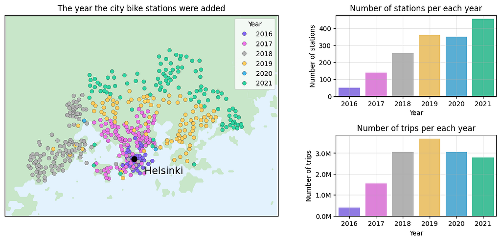
• How has the city bike station network expanded over the years?
• How has the number of trips changed over the years?

To address these questions, we start by plotting the station locations on a map by using the provided latitude and longitude coordinates.

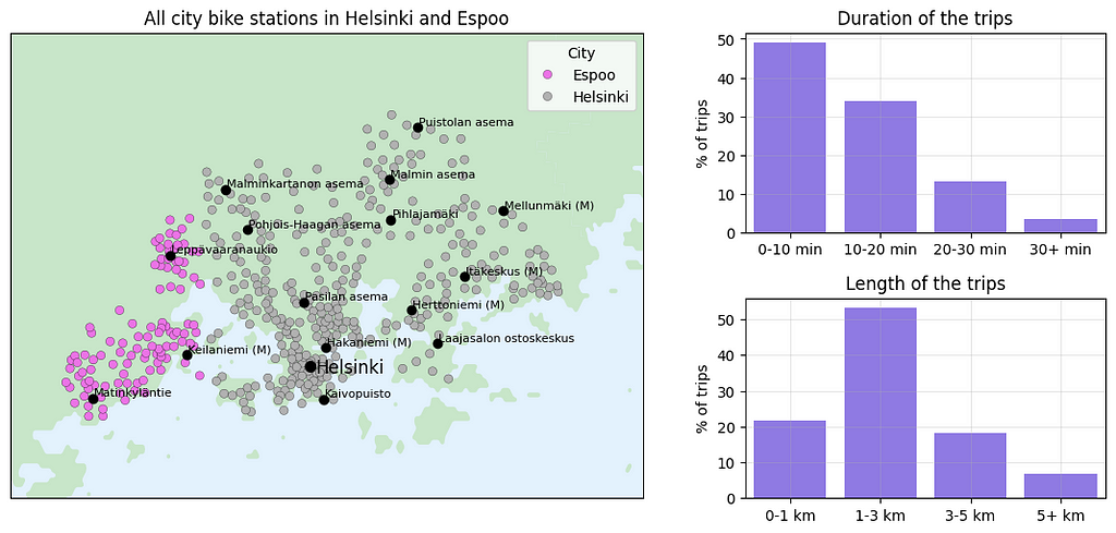
Next, we can analyze how the data have changed over the years.

To delve deeper into statistics derived from the city bike data, we will now incorporate hexagons in our analysis.

B. Using hexagon grid to analyze city bike data

Hexagons offer us a tool for detailed analysis of the city bike usage. The questions we aim to address using hexagons include:

• Where do we have a lot of city bike stations?
• In which areas of the city do we observe the highest number of departures or returns?
• What is the average trip length in different parts of Helsinki?

However, before tackling these questions, we need to decide the size of the hexagon we use in our analysis.

Let’s compute the station count within each hexagon and plot the hexagons with colors that reflect the number of stations within each respective hexagon:

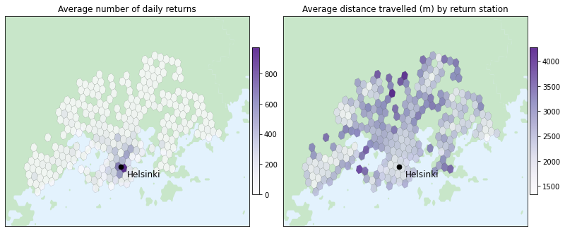
Hexagons help to visualize location-related insights, such as identifying the busiest parts of the town for the service. If we wouldn’t use hexagons, an alternative approach could involve calculating the average daily number of departures per station and plotting the result using circles of varying size, as shown in the figure below. However, the stations are so close to each other especially at the central Helsinki that it becomes challenging to accurately comprehend the daily number of departures.

With the hexagon grid we can also visualize various other insights from the data, such as the following graphs:

C. Selecting one hexagon and getting location specific insights

Sometimes we are interested in extracting more detailed insights from a specific region. By selecting one hexagon we can dive deeper into the data within that specific area and seek answers to questions such as:

• What are the peak usage times for city bikes in that area?
• How does bike usage vary between weekdays and weekends in that region?
• Where are users heading from that location?

To showcase how we could answer these questions, we opt for the following hexagon in the Helsinki city center:

Let’s begin examining the data from that specific area.

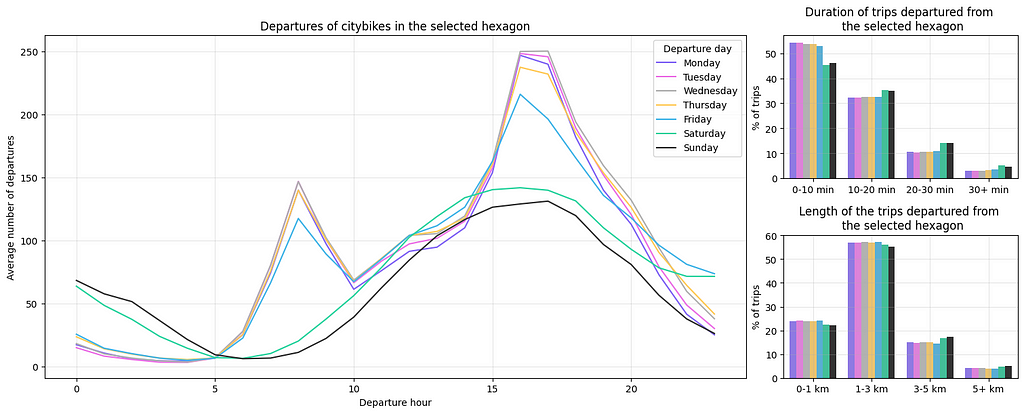
We can also visualize the destinations of trips originating from the selected hexagon to determine where users are heading from that area.

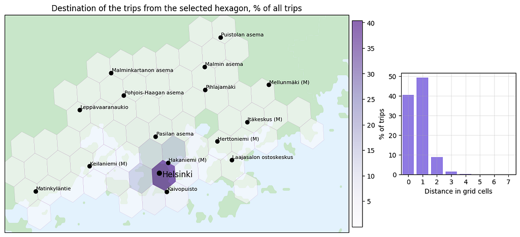
D. Selecting one location and analyzing data in the area around it

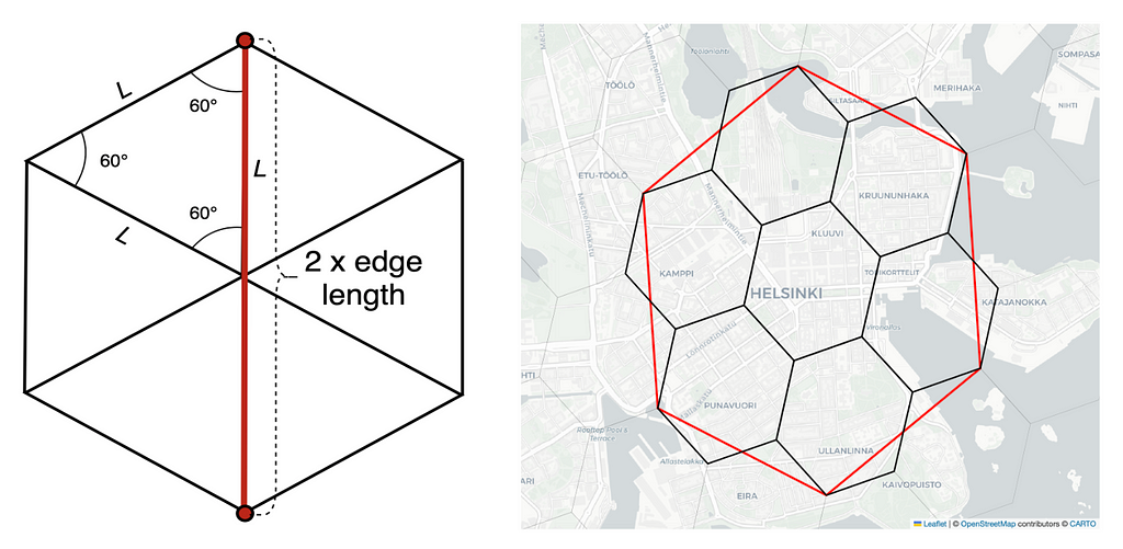
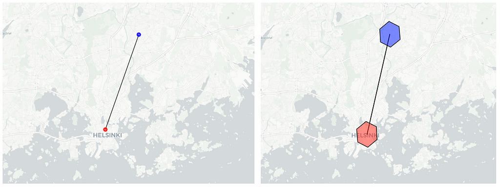
At times, we aim to gain insights around a specific location. For instance, we might want to understand city bike usage around a metro station that we frequently use, such as Kamppi metro station in this example. If we seek insights within a radius of approximately ~1 km, we might be tempted to choose the hexagon of resolution 7 containing the station, as the radius of that hexagon is roughly 1.4 km. However, as shown in the left image below, the selected station is not at the center of the hexagon, thus not effectively covering the ~1 km area around the data point.

Using the selected hexagons, we could analyze data around the desired data point.

E. Anonymising the location data

After obtaining hexagon indexes through geographic coordinates, we can omit the exact location data and exclusively utilise the H3 indexes. This aids in anonymizing the data, as there is no need to reveal the precise user location.

Issues with hexagons

The hexagon grid provided by the H3 library proves to be a useful tool for spatial data analysis. However, there are some challenges that arise when utilizing this hexagon grid, which we will elaborate on below.

From a mathematical perspective, the definition of hexagonal zones is entirely arbitrary. For this reason H3 hexagons lack alignment with any “natural elements,” such as streets, rivers, lakes, islands, highways, or train tracks. When employing the hexagon grid, data points are aggregated based on their proximity in straight-line distance. However, these points may not always be connected by roads, potentially resulting in the grouping of disparate locations into a single cluster. We show an example of this below.

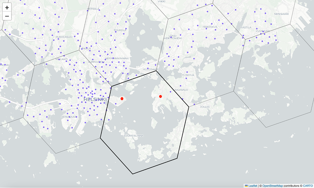
Another challenge arises if we aim to use the hexagons for anonymizing a user’s precise location. For example, instead of recording the user’s exact location, we could use hexagons of resolution 7 to indicate that the data point lies within an area with a radius of roughly 1.4 km. However, since the ideal hexagon resolution for analysis is often unknown, there may be a desire to link the data across various resolutions. But as the coarser hexagon only approximately contains its seven child hexagons, we might end up disclosing the location of a data point positioned close to the hexagon’s border more accurately than the specified 1.4 km radius. We demonstrate this in the image below.

Summary

• Uber’s global H3 hexagonal grid system is a user-friendly and practical tool for spatial data analysis. It can also help us to anonymise sensitive location data.
• H3 buckets location data points into hexagonal areas that cover the whole Earth with repetitive tiling. H3 library supports sixteen different hexagon resolutions, with the largest hexagons being ~1300km and the smallest only ~50m. From the different sizes of hexagons one must choose the resolution that best fits the purpose of the analysis.
• Each hexagon at finer resolution is roughly one seventh of the hexagon in coarser resolution. However, hexagons cannot be perfectly subdivided into seven smaller hexagons so the finer cells only approximately contain their parent cell. This means that the count of events in the parent cell might not be equal to the count of events in its children cells.
• Note that, hexagon grid lacks alignment with any “natural elements,” such as streets, rivers, lakes, islands, highways, or train tracks, so disparate locations might be grouped into a single cluster.

References:

• GitHub repository for the Helsinki city bike data analysis: https://github.com/sktahtin4/Helsinki-city-bikes
• Uber blog on H3: https://www.uber.com/en-FI/blog/h3/
• H3 documentation: https://h3geo.org/
• Table of statistics of the different hexagon resolutions: https://h3geo.org/docs/core-library/restable/
• More info on the global grid systems: http://webpages.sou.edu/~sahrk/sqspc/pubs/gdggs03.pdf
• Data viewer for the hexagons: https://wolf-h3-viewer.glitch.me
• HSL open data: https://www.hsl.fi/en/hsl/open-data

Exploring Location Data Using a Hexagon Grid was originally published in Towards Data Science on Medium, where people are continuing the conversation by highlighting and responding to this story.