An Intuitive View on Mutual Information

Layman’s guide to appreciating the concept of association

Recently I’ve been working on a project that aims to screen pairs of variables in the stock market, and see how they show enough correlation potential for us to deep-dive and research further.

Throughout my research, I’ve chanced upon many different methodologies; from the humble Spearman’s/Pearson linear correlation, to the more advanced non-linear methods using Time-Delay Embeddings and even Machine Learning techniques.

And that was when I chanced upon this robust and probabilistic concept known as Mutual Information that helps one to measure the level of association/dependence between two variables. This serves as a good Step 0 tool for model development or associative studies.

Scouring the web to understand further, I’ve realized that while there were excellent mathematical and statistical explanations, there weren’t many traces of intuitive insights on how and why Mutual Information works.

And therefore, here we are,

Welcome to my attempt at helping you break down and appreciate this statistical concept!

The Textbook Definition

Mutual Information is a measure of how much “information” you can get of one variable by observing another variable

I’m sure you’ve seen the above statement, or variants of it, throughout your own research. But what exactly is this “information” that they are talking about? How does it tell me that two variables are associated/dependent?

The definition becomes even more daunting when you look at the formulation:

Fret not! Let’s get into breaking down this concept into digestible chunks using a case study.

“Do people really use umbrellas only when it rains?”

said Bob, your drunk friend during a night out of festivities.

He insists that people carry umbrella only when they feel like it, and not because they need it to shelter them from the rain.

You think that that statement is ludicrous! It challenged every observation you made growing up; every notion of logic within your bones.

You decided to stalk Bob and observe him over the next 5 days during his vacation in tropical Singapore. You want to see if he really walks the talk and lives true to his bodacious claims.

You decide to do so using the concept of Mutual Information.

Bob vs Mutual Information

We can break down the Mutual Information formula into the following parts:

The x, X and y, Y

x and y are the individual observations/values that we see in our data. X and Y are just the set of these individual values. A good example would be as follows:

And assuming we have 5 days of observations of Bob in this exact sequence:

Individual/Marginal Probability

These are just the simple probability of observing a particular x or y in their respective sets of possible X and Y values.

Take x = 1 as an example: the probability is simply 0.4 (Bob carried an umbrella 2 out of 5 days of his vacation).

Joint Probability

This is the probability of observing a particular x and y from the joint probability of (X, Y). The joint probability (X, Y) is simply just the set of paired observations. We pair them up according to their index.

In our case with Bob, we pair the observations up based on which day they occurred.

You may be tempted to jump to a conclusion after looking at the pairs:

Since there are equal-value pairs occurring 80% of the time, it clearly means that people carry umbrellas BECAUSE it is raining!

Well I’m here to play the devil’s advocate and say that that may just be a freakish coincidence:

If the chance of rain is very low in Singapore, and, independently, the likelihood of Bob carrying umbrella is also equally low (because he hates holding extra stuff), can you see that the odds of having (0,0) paired observations will be very high naturally?

So what can we do to prove that these paired observations are not by coincidence?

Joint Versus Individual Probabilities

We can take the ratio of both probabilities to give us a clue on the “extent of coincidence”.

In the denominator, we take the product of both individual probabilities of a particular x and particular y occurring. Why did we do so?

Peering into the humble coin toss

Recall the first lesson you took in statistics class: calculating the probability of getting 2 heads in 2 tosses of a fair coin.

• 1st Toss [ p(x) ]: There’s a 50% chance of getting heads
• 2nd Toss [ p(y) ]: There’s still a 50% chance of getting heads, since the outcome is independent of what happened in the 1st toss
• The above 2 tosses make up your individual probabilities
• Therefore, the theoretical probability of getting both heads in 2 independent tosses is 0.5 * 0.5 = 0.25 ( p(x).p(y) )

And if you actually do maybe 100 sets of that double-coin-toss experiment, you’ll likely see that you get the (heads, heads) result 25% of the time. The 100 sets of experiment is actually your (X, Y) joint probability set!

Hence, when you take the ratio of joint versus combined-individual probabilities, you get a value of 1.

This is actually the real expectation for independent events: the joint probability of a specific pair of values occurring is exactly equal to the product of their individual probabilities! Just like what you were taught in fundamental statistics.

Now imagine that your 100-set experiment yielded (heads, heads) 90% of the time. Surely that can’t be a coincidence…

You expected 25% since you know that they are independent events, yet what was observed is an extreme skew of this expectation.

To put this qualitative feeling into numbers, the ratio of probabilities is now a whopping 3.6 (0.9 / 0.25), essentially 3.6x more frequent than we expected.

As such, we start to think that maybe the coin tosses were not independent. Maybe the result of the 1st toss might actually have some unexplained effect on the 2nd toss. Maybe there is some level of association/dependence between 1st and 2nd toss.

That is what Mutual Information tries to tells us!

Expected Value of Observations

For us to be fair to Bob, we should not just look at the times where his claims are wrong, i.e. calculate the ratio of probabilities of (0,0) and (1,1).

We should also calculate the ratio of probabilities for when his claims are correct, i.e. (0,1) and (1,0).

Thereafter, we can aggregate all 4 scenarios in an expected value method, which just means “taking the average”: aggregate up all ratio of probabilities for each observed pair in (X, Y), then divide it by the number of observations.

That is the purpose of these two summation terms. For continuous variables like my stock market example, we will then use integrals instead.

Logarithm of Ratios

Similar to how we calculate the probability of getting 2 consecutive heads for the coin toss, we are also now calculating the additional probability of seeing the 5 pairs that we observed.

For the coin toss, we calculate by multiplying the probabilities of each toss. For Bob, it’s the same: the probabilities have multiplicative effect on each other to give us the sequence that we observed in the joint set.

With logarithms, we turn multiplicative effects into additive ones:

Converting the ratio of probabilities to their logarithmic variants, we can now simply just calculate the expected value as described above using summation of their logarithms.

Feel free to use log-base 2, e, or 10, it does not matter for the purposes of this article.

Putting It All Together

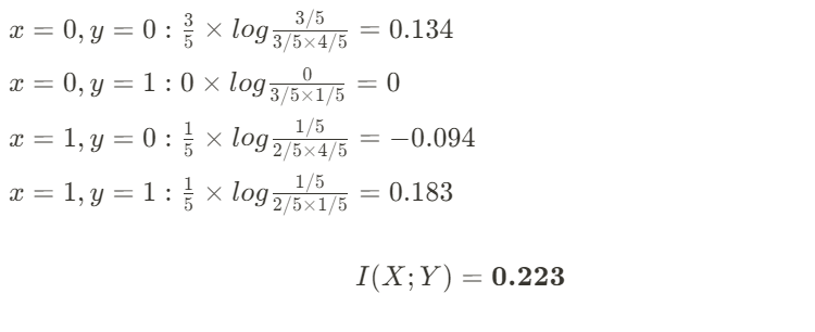
Let’s now prove Bob wrong by calculating the Mutual Information. I will use log-base e (natural logarithm) for my calculations:

So what does the value of 0.223 tell us?

Let’s first assume Bob is right, and that the use of umbrellas are independent from presence of rain:

• We know that the joint probability will exactly equal the product of the individual probabilities.
• Therefore, for every x and y permutation, the ratio of probabilities = 1.
• Taking the logarithm, that equates to 0.
• Thus, the expected value of all permutations (i.e. Mutual Information) is therefore 0.

But since the Mutual Information score that we calculated is non-zero, we can therefore prove to Bob that he is wrong!

Beyond Linear Correlation

Because Mutual Information is a probabilistic measure of association/dependence, it can work for non-linear correlation studies as well!

Take for example two variables X and Y:

Calculating their Mutual Information score, Spearman’s correlation score, and plotting, we get the following:

Relying on Spearman’s correlation alone, we would think that these 2 variables have nothing to do with each other, but we know for a fact that they are deterministically related (based on my formula above)!

The non-zero Mutual Information score hints us to look deeper, albeit not giving us the explicit form of relation.

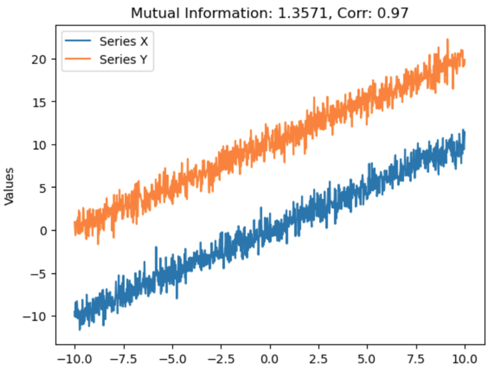
It is also robust enough to work on strictly linear correlations:

So, if you are ever unsure what kind of correlation you are expecting going into an X-vs-Y analysis, you can try out Mutual Information as a step zero!

My “Layman” Definition of Mutual Information

With the above examples and breakdown, I hope I managed to help you guys get an intuitive understanding what Mutual Information is and how it works.

If it helps you further, I prefer to summarize Mutual Information as follows:

Mutual Information gives us the additional probability of x and y happening at the same time due to other factors above just their chance of co-occurring.

Mutual Information is very useful in areas such as Feature Selection before building your Machine Learning models, and even text association analyses when used with text embeddings. Therefore, it is paramount that we truly know how it works before adopting it for its myriad of uses.

With your newfound intuition and understanding, I believe you will be able to find other pockets of opportunities to apply this versatile concept as I will with my stock market ventures!

An Intuitive View on Mutual Information was originally published in Towards Data Science on Medium, where people are continuing the conversation by highlighting and responding to this story.