Understanding the mathematical background of graph neural networks and implementation for a regression problem in pytorch
Introduction
Interconnected graphical data is all around us, ranging from molecular structures to social networks and design structures of cities. Graph Neural Networks (GNNs) are emerging as a powerful method of modelling and learning the spatial and graphical structure of such data. It has been applied to protein structures and other molecular applications such as drug discovery as well as modelling systems such as social networks. Recently the standard GNN has been combined with ideas from other ML models to develop exciting innovative applications. One such development is the integration of GNN with sequential models — Spatio-Temporal GNN that is able to capture both the temporal and spatial (hence the name) dependences of data, this alone could be applied to a number of challenges/problems in industry/research.
Despite the exciting developments in GNN, there are very few resources on the topic which makes it inaccessible to many. In this short article, I want to provide a brief introduction to GNN covering both the mathematical description as well as a regression problem using the pytorch library. By unraveling the principles behind GNNs, we unlock a deeper comprehension of their capabilities and applications.
Mathematical Description of GNNs
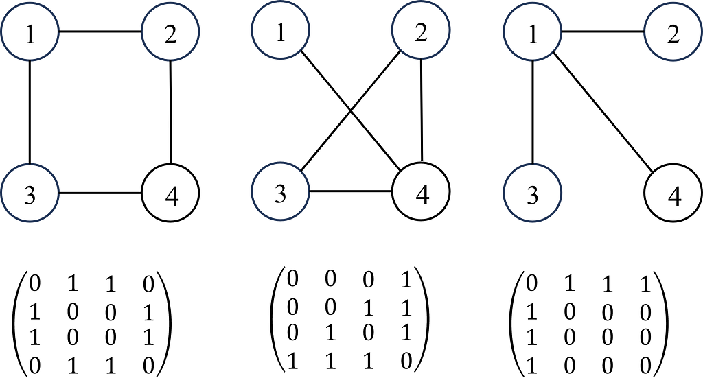
A graph G can be defined as G = (V, E), where V is the set of nodes, and E are the edges between them. A graph is often represented by an adjacency matrix, A, which represents the presence or absence of edges between nodes i.e. aij takes values of 1 to indicate an edge (connection) between nodes i and j or 0 otherwise. If a graph has n nodes, A has a dimension of (n × n). The adjacency matrix is demonstrated in Figure 1.

Each node (and edges! But we’ll come back to this later for simplicity) will have a set of features (e.g. if the node is a person, the features will be age, gender, height, job etc). If each node has f features, then the feature matrix X is (n × f). In some problems, each node may also have a target label which maybe a set of categorical labels or numerical values (shown in Figure 2).
Single Node Calculations
To learn the interdependence between any node and its neighbours, we need to consider the features of its neighbours. This is what enables GNNs to learn the structural representation of the data through a graph. Consider a node j with Nj neighbours, GNNs transform the features from each neighbour, aggregate them and then update node i’s feature space. Each of these steps are described as follows.
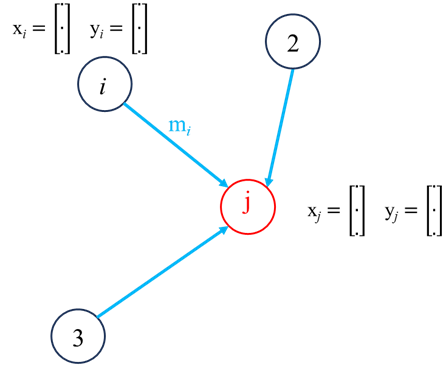
Neighbour feature transformation could be done a number of ways such as passing through an MLP network or by linear transformation such as

where w and b represent the weights and bias of the transformation. Information aggregation, the information from each neighboring nodes are then aggregated:

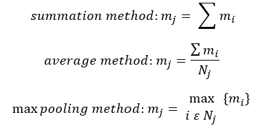
The nature of the aggregation step could be a number of different methods such as summation, averaging, min/max pooling and concatenation:
Following the aggregation step, the final step is to update node j:

This updated could be done using MLP with the concatenated node features and neighbour information aggregation (mj) or we could use linear transformation i.e.

Where U is a learnable weights matrix that combines the original node features (xj) with aggregated neighbour features (mj) through a non-linear activation function (ReLU in this case). This is it for the process of updating a single node in a single layer, the same process is applied to all other nodes in the graph, mathematically, this can be presented using the Adjacency matrix.
Graph Level Calculation
For a graph with n nodes and each node has f features, we can concatenate all the features in a single matrix:

The neighbour feature transformation and aggregation steps can therefore be written as:

Where I is the identity matrix, this helps to include the each nodes own features too, otherwise, we are only considering the transformed features from the node j’s neighbours and not it’s own features. One final step is to normalise each node based on the number of connections i.e. for node j with Nj connections, the feature transformation can be done as:

The equation above can be adjusted as:

Where D is the degree matrix, a diagonal matrix of number of connections for each node. However, more commonly, this normalisation step is done as

This is the graph convolution network (GCN) method that enables GNN to learn the structure and relationship between nodes. However, an issue with GCN is that the weight vector for neighbour feature transformation is shared across all neighbours i.e. all neighbours are considered equal, but this is usually not the case so not a good representative of real systems. To address is, graph attention network (GATs) can be used to compute the importance of a neighbour’s feature to the target node, allowing the different neighbours to contribute differently to the feature update of the target node based on their relevance. The attention coefficients are determined using a learnable matrix as follows:

Where W is the shared learnable feature linear transformation, Wa is a learnable weight vector and eij is the raw attention score indicating importance of node i’s features to node j. The attention score is normalised using the SoftMax function:

Now the feature aggregation step can be calculated using the attention coefficients:

This is it for a single layer, we can build multiple layers to increase the complexity of the model, this is demonstrated in Figure 3. Increasing the number of layers will allow the model to learn more global features and also capture more complex relationships, however, it is also likely to overfit so regularisation techniques should always be used to prevent this.
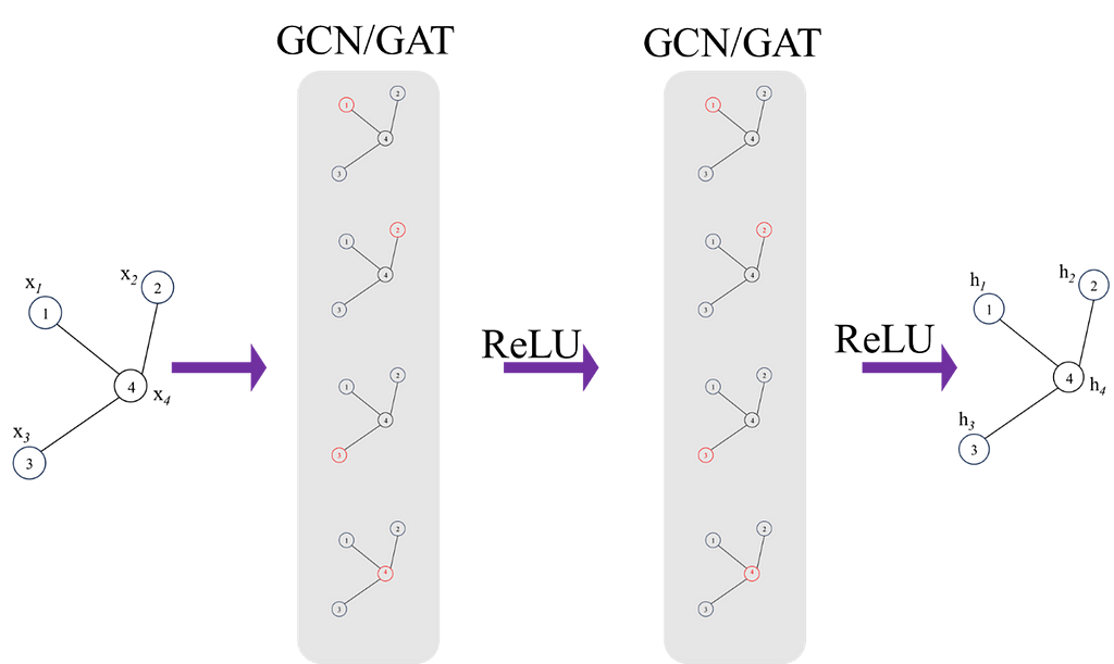
Finally, once final feature vectors for all nodes are obtained from the network, a feature matrix, H can be formed:

This feature matrix can be used to do a number of tasks e.g. node or graph classification. This brings us to the end of introduction into the mathematical description of GCN/GATs.
GCN Regression Example
Let’s implement a regression example where the aim is to train a network to predict the value of a node given the value of all other nodes i.e. each node has a single feature (which is a scalar value). The aim of this example is to leverage the inherent relational information encoded in the graph to accurately predict numerical values for each node. The key thing to note is that we input the numerical value for all nodes except the target node (we mask the target node value with 0) then predict the target node’s value. For each data point, we repeat the process for all nodes. Perhaps this might come across as a bizarre task but lets see if we can predict the expected value of any node given the values of the other nodes. The data used is the corresponding simulation data to a series of sensors from industry and the graph structure I have chosen in the example below is based on the actual process structure. I have provided comments in the code to make it easy to follow. You can find a copy of the dataset here (Note: this is my own data, generated from simulations).
This code and training procedure is far from being optimised but it’s aim is to illustrate the implementation of GNNs and get an intuition for how they work. An issue with the currently way I have done that should definitely not be done this way beyond learning purposes is the masking of node feature value and predicting it from the neighbours feature. Currently you’d have to loop over each node (not very efficient), a much better way to do is the stop the model from include it’s own features in the aggregation step and hence you wouldn’t need to do one node at a time but I thought it is easier to build intuition for the model with the current method:)
Preprocessing Data
Importing the necessary libraries and Sensor data from CSV file. Normalise all data in the range of 0 to 1.
import pandas as pd
import torch
from torch_geometric.data import Data, Batch
from sklearn.preprocessing import StandardScaler, MinMaxScaler
from sklearn.model_selection import train_test_split
import numpy as np
from torch_geometric.data import DataLoader

# load and scale the dataset
df = pd.read_csv('SensorDataSynthetic.csv').dropna()
scaler = MinMaxScaler()
df_scaled = pd.DataFrame(scaler.fit_transform(df), columns=df.columns)
Defining the connectivity (edge index) between nodes in the graph using a PyTorch tensor — i.e. this provides the system’s graphical topology.
nodes_order = [
    'Sensor1', 'Sensor2', 'Sensor3', 'Sensor4',
    'Sensor5', 'Sensor6', 'Sensor7', 'Sensor8'
]

# define the graph connectivity for the data
edges = torch.tensor([
    [0, 1, 2, 2, 3, 3, 6, 2],  # source nodes
    [1, 2, 3, 4, 5, 6, 2, 7]   # target nodes
], dtype=torch.long)
The Data imported from csv has a tabular structure but to use this in GNNs, it must be transformed to a graphical structure. Each row of data (one observation) is represented as one graph. Iterate through Each Row to Create Graphical representation of the data
A mask is created for each node/sensor to indicate the presence (1) or absence (0) of data, allowing for flexibility in handling missing data. In most systems, there may be items with no data available hence the need for flexibility in handling missing data. Split the data into training and testing sets
graphs = []

# iterate through each row of data to create a graph for each observation
# some nodes will not have any data, not the case here but created a mask to allow us to deal with any nodes that do not have data available
for _, row in df_scaled.iterrows():
    node_features = []
    node_data_mask = []
    for node in nodes_order:
        if node in df_scaled.columns:
            node_features.append([row[node]])
            node_data_mask.append(1) # mask value of to indicate present of data
        else:
            # missing nodes feature if necessary
            node_features.append(2)
            node_data_mask.append(0) # data not present

    node_features_tensor = torch.tensor(node_features, dtype=torch.float)
    node_data_mask_tensor = torch.tensor(node_data_mask, dtype=torch.float)


    # Create a Data object for this row/graph
    graph_data = Data(x=node_features_tensor, edge_index=edges.t().contiguous(), mask = node_data_mask_tensor)
    graphs.append(graph_data)


#### splitting the data into train, test observation
# Split indices
observation_indices = df_scaled.index.tolist()
train_indices, test_indices = train_test_split(observation_indices, test_size=0.05, random_state=42)

# Create training and testing graphs
train_graphs = [graphs[i] for i in train_indices]
test_graphs = [graphs[i] for i in test_indices]
Graph Visualisation
The graph structure created above using the edge indices can be visualised using networkx.
import networkx as nx
import matplotlib.pyplot as plt

G = nx.Graph()
for src, dst in edges.t().numpy():
    G.add_edge(nodes_order[src], nodes_order[dst])

plt.figure(figsize=(10, 8))
pos = nx.spring_layout(G)
nx.draw(G, pos, with_labels=True, node_color='lightblue', edge_color='gray', node_size=2000, font_weight='bold')
plt.title('Graph Visualization')
plt.show()
Model Definition
Let’s define the model. The model incorporates 2 GAT convolutional layers. The first layer transforms node features to an 8 dimensional space, and the second GAT layer further reduces this to an 8-dimensional representation.
GNNs are highly susceptible to overfitting, regularation (dropout) is applied after each GAT layer with a user defined probability to prevent over fitting. The dropout layer essentially randomly zeros some of the elements of the input tensor during training.
The GAT convolution layer output results are passed through a fully connected (linear) layer to map the 8-dimensional output to the final node feature which in this case is a scalar value per node.
Masking the value of the target Node; as mentioned earlier, the aim of this of task is to regress the value of the target node based on the value of it’s neighbours. This is the reason behind masking/replacing the target node’s value with zero.
from torch_geometric.nn import GATConv
import torch.nn.functional as F
import torch.nn as nn

class GNNModel(nn.Module):
    def __init__(self, num_node_features):
        super(GNNModel, self).__init__()
        self.conv1 = GATConv(num_node_features, 16)
        self.conv2 = GATConv(16, 8)
        self.fc = nn.Linear(8, 1)  # Outputting a single value per node

    def forward(self, data, target_node_idx=None):
        x, edge_index = data.x, data.edge_index
        edge_index = edge_index.T
        x = x.clone()

        # Mask the target node's feature with a value of zero!
        # Aim is to predict this value from the features of the neighbours
        if target_node_idx is not None:
            x[target_node_idx] = torch.zeros_like(x[target_node_idx])

        x = F.relu(self.conv1(x, edge_index))
        x = F.dropout(x, p=0.05, training=self.training)
        x = F.relu(self.conv2(x, edge_index))
        x = F.relu(self.conv3(x, edge_index))
        x = F.dropout(x, p=0.05, training=self.training)
        x = self.fc(x)

        return x
Training the model
Initialising the model and defining the optimiser, loss function and the hyper parameters including learning rate, weight decay (for regularisation), batch_size and number of epochs.
model = GNNModel(num_node_features=1)
batch_size = 8
optimizer = torch.optim.Adam(model.parameters(), lr=0.0002, weight_decay=1e-6)
criterion = torch.nn.MSELoss()
num_epochs = 200
train_loader = DataLoader(train_graphs, batch_size=1, shuffle=True)
model.train()
The training process is fairly standard, each graph (one data point) of data is passed through the forward pass of the model (iterating over each node and predicting the target node. The loss from the prediction is accumulated over the defined batch size before updating the GNN through backpropagation.
for epoch in range(num_epochs):
    accumulated_loss = 0
    optimizer.zero_grad()
    loss = 0
    for batch_idx, data in enumerate(train_loader):
        mask = data.mask
        for i in range(1,data.num_nodes):
            if mask[i] == 1:  # Only train on nodes with data
                output = model(data, i)  # get predictions with the target node masked
                                         # check the feed forward part of the model
                target = data.x[i]
                prediction = output[i].view(1)
                loss += criterion(prediction, target)
        #Update parameters at the end of each set of batches
        if (batch_idx+1) % batch_size == 0 or (batch_idx +1 ) == len(train_loader):
            loss.backward()
            optimizer.step()
            optimizer.zero_grad()
            accumulated_loss += loss.item()
            loss = 0

    average_loss = accumulated_loss / len(train_loader)
    print(f'Epoch {epoch+1}, Average Loss: {average_loss}')
Testing the trained model
Using the test dataset, pass each graph through the forward pass of the trained model and predict each node’s value based on it’s neighbours value.
test_loader = DataLoader(test_graphs, batch_size=1, shuffle=True)
model.eval()

actual = []
pred = []

for data in test_loader:
    mask = data.mask
    for i in range(1,data.num_nodes):
        output = model(data, i)
        prediction = output[i].view(1)
        target = data.x[i]

        actual.append(target)
        pred.append(prediction)
Visualising the test results
Using iplot we can visualise the predicted values of nodes against the ground truth values.
import plotly.graph_objects as go
from plotly.offline import iplot

actual_values_float = [value.item() for value in actual]
pred_values_float = [value.item() for value in pred]


scatter_trace = go.Scatter(
    x=actual_values_float,
    y=pred_values_float,
    mode='markers',
    marker=dict(
        size=10,
        opacity=0.5,
        color='rgba(255,255,255,0)',
        line=dict(
            width=2,
            color='rgba(152, 0, 0, .8)',
        )
    ),
    name='Actual vs Predicted'
)

line_trace = go.Scatter(
    x=[min(actual_values_float), max(actual_values_float)],
    y=[min(actual_values_float), max(actual_values_float)],
    mode='lines',
    marker=dict(color='blue'),
    name='Perfect Prediction'
)

data = [scatter_trace, line_trace]

layout = dict(
    title='Actual vs Predicted Values',
    xaxis=dict(title='Actual Values'),
    yaxis=dict(title='Predicted Values'),
    autosize=False,
    width=800,
    height=600
)

fig = dict(data=data, layout=layout)

iplot(fig)
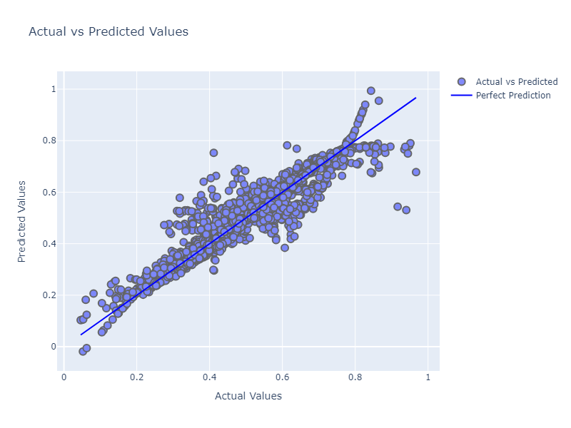
Despite a lack of fine tuning the model architecture or hyperparameters, it has done a decent job actually, we could tune the model further to get improved accuracy.
This brings us to the end of this article. GNNs are relatively newer than other branches of machine learning, it will be very exciting to see the developments of this field but also it’s application to different problems. Finally, thank you for taking the time to read this article, I hope you found it useful in your understanding of GNNs or their mathematical background.
Unless otherwise noted, all images are by the author
Structure and Relationships: Graph Neural Networks and a Pytorch Implementation was originally published in Towards Data Science on Medium, where people are continuing the conversation by highlighting and responding to this story.
Originally appeared here:
Structure and Relationships: Graph Neural Networks and a Pytorch Implementation
