Visualizing Dynamical Behavior in Agent-Based Models

And encountering emergent complexity along the way

In my research into streamlining strategic knowledge extraction in game theoretic problems, I recently realized that I needed a better way to simply and intuitively visualize the behavior of agents with defined dynamical behavior.

This led me to build a simple library for visualizing agent behavior as an animation using PyPlot. But before jumping into the tutorial, here’s a quick catch-up on the core concepts at play here.

A Quick Primer on Dynamical Agent-Based Modeling

Agent based modeling (ABM) offers an excellent way to simulate players in many game theoretic environments. It lets us model and study the behavior and cognitive processes of each individual player, rather than just analyzing trends. When it isn’t practical to represent agents using simplistic binary state machines like cellular automata grids, ABM lets us capture scenarios by representing the agents’ positions in a dimensional space, where each dimension has its own unique rules.

Agents in Position and State Space

By utilizing both spatial and state dimensions we can accurately model proximity as well as incorporate attributes that allow for subtle interactions, such as similarity in characteristics. Furthermore, storing the “positions” of agents in state space allow us to keep track of and compare detailed and dynamic state information about agents (i.e. a player’s fatigue in a model of football).

Compared to network models, wherein the existence of connections between two objects indicate relationships, position-state-space information lets us to define and explore more complex and higher-dimensional relationships between agents. In this paradigm, Euclidean distance in state-space could represent a strong measure of the state similarity between two agents.

Dynamical Systems Theory for Behavior and Interaction

We can make such a model even more powerful by using dynamical systems theory to describe how the state of one agent influences those of others. It provides a robust way to define rules a system’s evolution over time.

In socioeconomic systems, differential equations can be used to model communication, mimicry, and more complex adaptive processes, as well as describe how individual actions can produce group dynamics.

Visualization Needs in Time and Space

For my problem, I wanted to be able see the position of each agent and its movement over time at a glance, and some basic state information (i.e. one or two variables per agent).

There are currently several libraries that meet the need for visualizing ABMs, including NetLogo and Mesa (for Python). However, they are built primarily for visualizing discrete-space, rather than continuous-space models. For my purposes, I was interested in the latter, and so began the side quest. If you’d like to follow along or test out the code for yourself, it’s all stored at github.com/dreamchef/abm-viz.

Building the Classes and Animation in Python

For starters, I needed to represent and store the agents and the world, and their state and dynamics. I chose to do this using Python classes. I defined an Agent class with a set of variables that I thought might be relevant to many possible modeling tasks. I also defined a plottable circle object (with PyPlot) for each agent within the class structure.

class Agent:

    def __init__(self, index, position, velocity, empathy=1, ... dVision=0, age=0, plotSize=10):
        
        self.index = index
        self.velocity = np.array(velocity)
        self.empathy = empathy
        ...
        self.dVision = dVision
        self.color = HSVToRGB([self.species,1,1])
        self.plotSize=plotSize

        self.pltObj = plt.Circle(self.position, self.plotSize, color=self.color)

Then, after a bit of experimentation, I found that it in the spirit of good objected-oriented programming principles, it would be best to define a World (think game or system) class as well. In included both the state information for the world and the information for the plots and axes in the class structure:

class World:

    def __init__(self,population=1,spawnSize=400,worldSize=1200,worldInterval=300,arrows=False,agentSize=10):
        
        self.agents = []
        self.figure, self.ax = plt.subplots(figsize=(12,8))
        self.ax.set_xlim(-worldSize/2, worldSize/2)
        self.ax.set_ylim(-worldSize/2, worldSize/2)

        self.worldInterval = worldInterval
        self.worldSize = worldSize
        self.arrows = arrows
        self.agentSize = agentSize

        for i in range(population):

            print(i)

            newAgent = Agent(index=i, position=[rand()*spawnSize - spawnSize/2, rand()*spawnSize - spawnSize/2],
                                     velocity=[rand()*spawnSize/10 - spawnSize/20, rand()*spawnSize/10 - spawnSize/20], plotSize = self.agentSize)

            self.agents.append(newAgent)
            self.ax.add_patch(newAgent.pltObj)

            print('Created agent at',newAgent.position,'with index',newAgent.index)

        self.spawnSize = spawnSize

I wrote this class so that the programmer can simply specify the desired number of agents (along with other parameters such as a world size and spawn area size) rather than manually creating and adding agents in the main section.

With this basic structure defined and agents being generated with randomized positions and initial velocities in the world, I then used PyPlot library’s animation features to create a method which would begin the visualization:

def start(self):

        ani = animation.FuncAnimation(self.figure, self.updateWorld, frames=100, interval=self.worldInterval, blit=True)

        plt.show()

This function references the figure, stored in the World instance, some specifications for the speed and length of the animation, and an update function, which is also defined in the World class:

def updateWorld(self,x=0):

        pltObjects = []

        for agent in self.agents:

            agent.updatePosition(self.agents, self.worldSize)
            agent.pltObj.center = agent.position
            pltObjects.append(agent.pltObj)

            if self.arrows is True:
           
                velocityArrow = plt.Arrow(agent.position[0], agent.position[1], agent.velocity[0], agent.velocity[1], width=2, color=agent.color)

                self.ax.add_patch(velocityArrow)

                pltObjects.append(velocityArrow)

        return pltObjects

The World.updatePosition function simply added each agent’s static velocity to the current position. This preliminary work was able to generate simple animations like this:

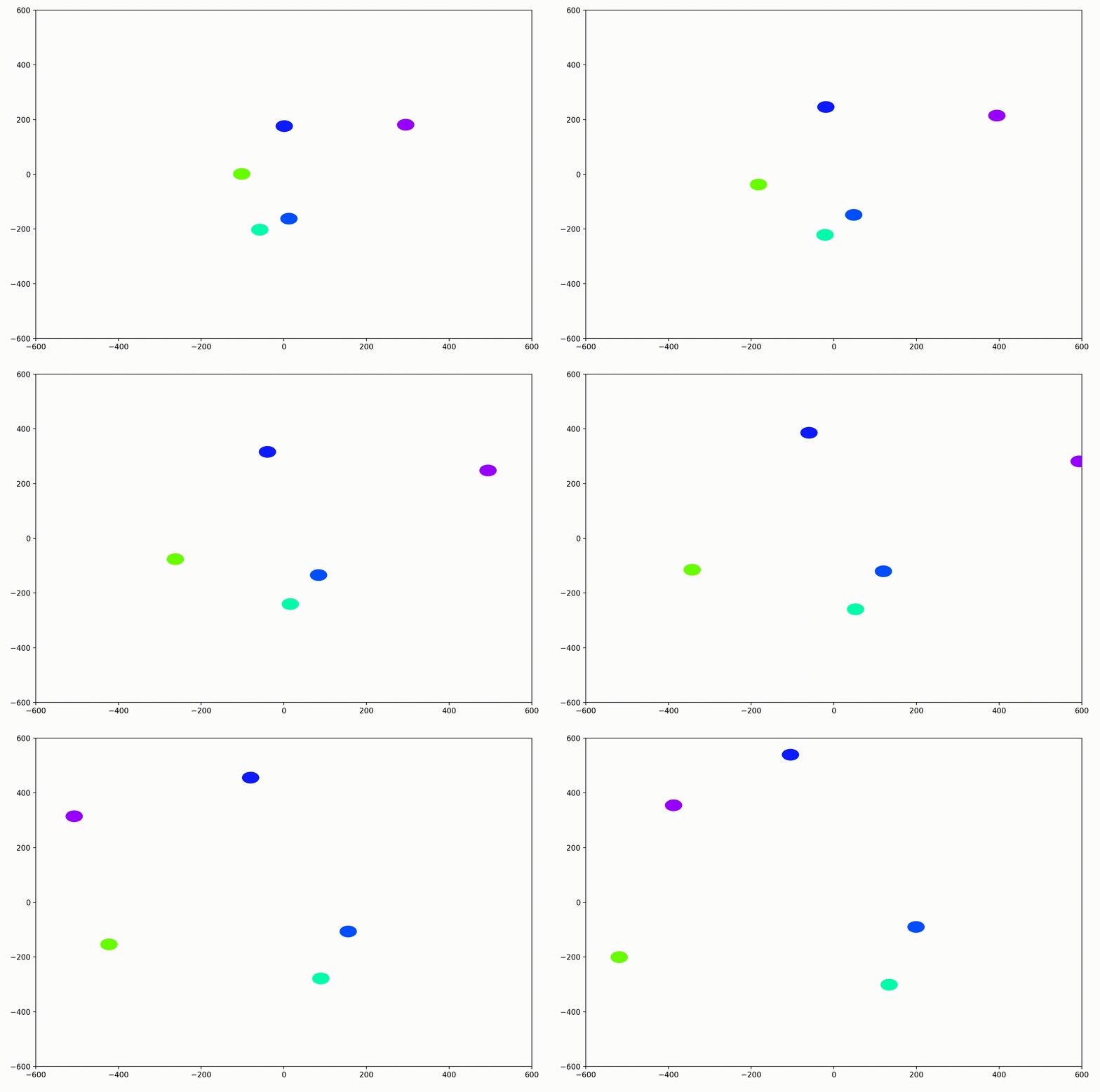
With this basic functionality, we’d now like to be able to visualize more interesting dynamics.

Visualizing “Social” Dynamic Behavior

I first chose to define a dynamic where each agent would change its direction of movement based on the average direction of movement of other agents around it. In equation form:

I encoded the dynamic in Python via an Agent.updatePosition() and an Agent.updateVelocity() method, which are run on each animation frame:

def updatePosition(self, agents, worldSize):

        self.updateVelocity(agents)

        self.position += self.velocity

        ...

    def updateVelocity(self, agents):

        herd_velocity = self.herdVelocity(agents)

        herd_magnitude = np.linalg.norm(herd_velocity)
        self_magnitude = np.linalg.norm(self.velocity)

        if herd_magnitude > 0.1:
            
            herd_unit_velocity = herd_velocity/herd_magnitude

            self.velocity += herd_unit_velocity

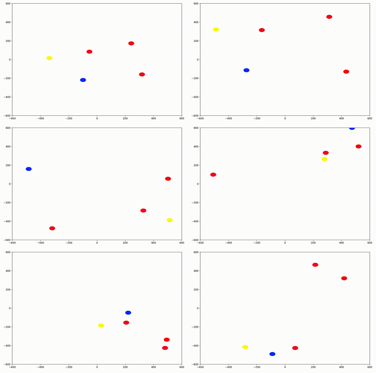
In the PyPlot animation below, the agents begin with very different velocities, but quickly adjust and begin traveling in the same direction. In this case, the average direction was roughly upward in the Y-direction at first.

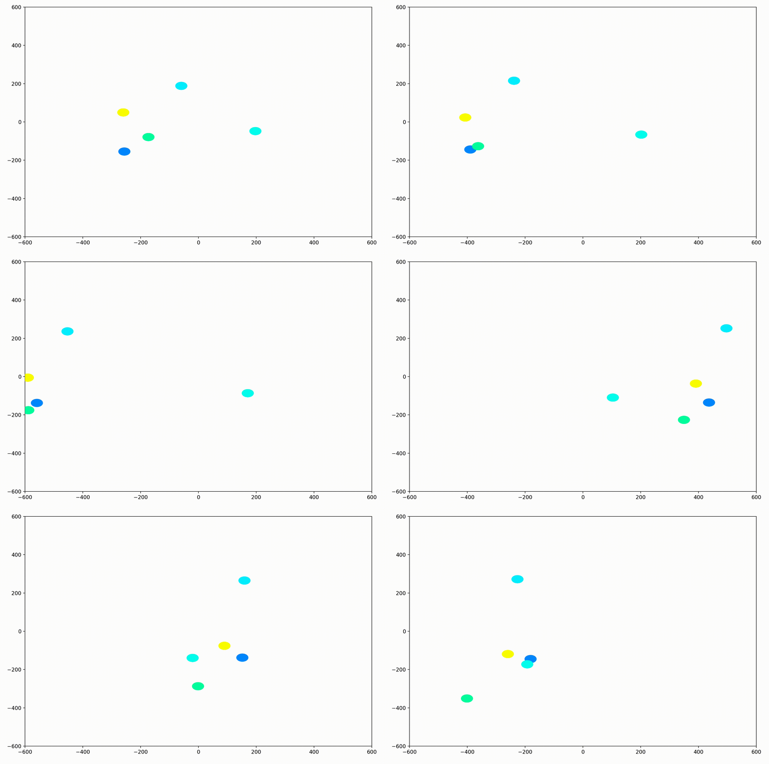
This time, the group had initialized with a roughly leftward velocity with one “straggling”, who quickly adjusts.

Displaying Velocity Vectors

Next I realized it would be helpful to see the velocity of the agents more clearly, so I implemented arrows to show each agent’s magnitude and direction:

velocityArrow = plt.Arrow(agent.position[0], agent.position[1], agent.velocity[0], agent.velocity[1], width=2, color=agent.color)
self.ax.add_patch(velocityArrow)
pltObjects.append(velocityArrow)

That modification gave more helpful animations like this one. We can still notice the converging-velocities dynamic at a glance, but see the rates of acceleration more clearly now as well.

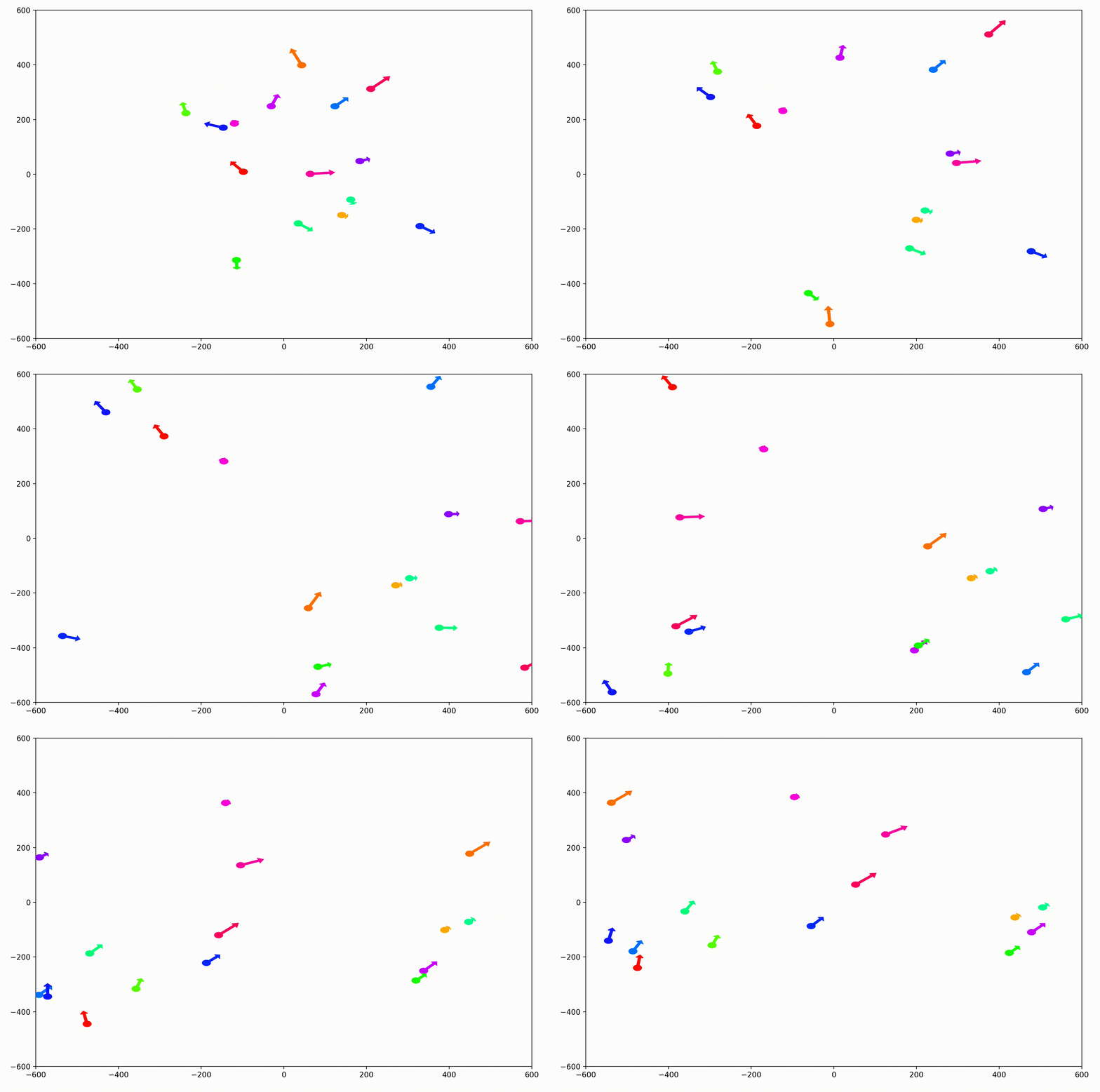
For the animation above, I also adjusting the dynamic to be dependent on a sight range variable. In other words, agents only adjust their velocities to match agents that are nearby (within 300 units in this case).

I also modified the code so that each agent would only modify its direction of movement, not its speed. Keep this in mind for the next section.

More Complex, State-Wise Dynamics

Up until this point, I had only implemented dynamics which considered the positions and velocities of each agent. But as I alluded to in the overview section, consider non-spatial, state information as well can make our modeling approach much more generalizable.

Using Agent Hue and Saturation To Represent State Variables

I made use an auxiliary state tied to the RGB color of each agent. Foreshadowing the evolutionary game theoretic goals of my research, I call this the agent “species”, and implement it as follows.

In the Agent.__init__ method, I added random species generation and individual mapping to the color of the agent’s marker on the plot:

self.species = rand()
self.color = HSVToRGB([self.species,1,1])
self.pltObj = plt.Circle(self.position, self.plotSize, color=self.color)

Specifically, I assigned this to the hue of the object, to reserve the saturation (roughly grey-ness) for other variables of potential interest (i.e. remaining lifespan or health). This practice of dividing hue and saturation has precedent in the visualization of complex-valued functions, which I go into in this article.

Dependence of Acceleration on Species State Variable

With examples of herding behavior in nature that occurs between animals of the same species, but not between those of differing species, I decided to change our toy dynamics to consider species. This change meant that each agent will only modify its direction for agents that are sufficiently close in the world and sufficiently similar in species (i.e. similarly colored circles).

Now, this is where things, began to get very, very interesting. Before you continue reading, ask yourself:

• What behavior do you expect to see in the next animation?

A relatively naive experimenter (such as myself most of the time) would expect agents to organize themselves by species and travel in herds, with each herd tending to travel in different directions and mostly ignoring each other. To see if either of us is right, let’s continue.

To encode this behavior I modified the calculation of herd velocity with respect to an agent in the following way:

herd_velocity += neighbor.velocity * (0.5-np.sqrt(abs(self.species-neighbor.species)))

That change resulted in animations like this one. To see the interesting behavior here, I started recording this about 20 seconds into the animation.

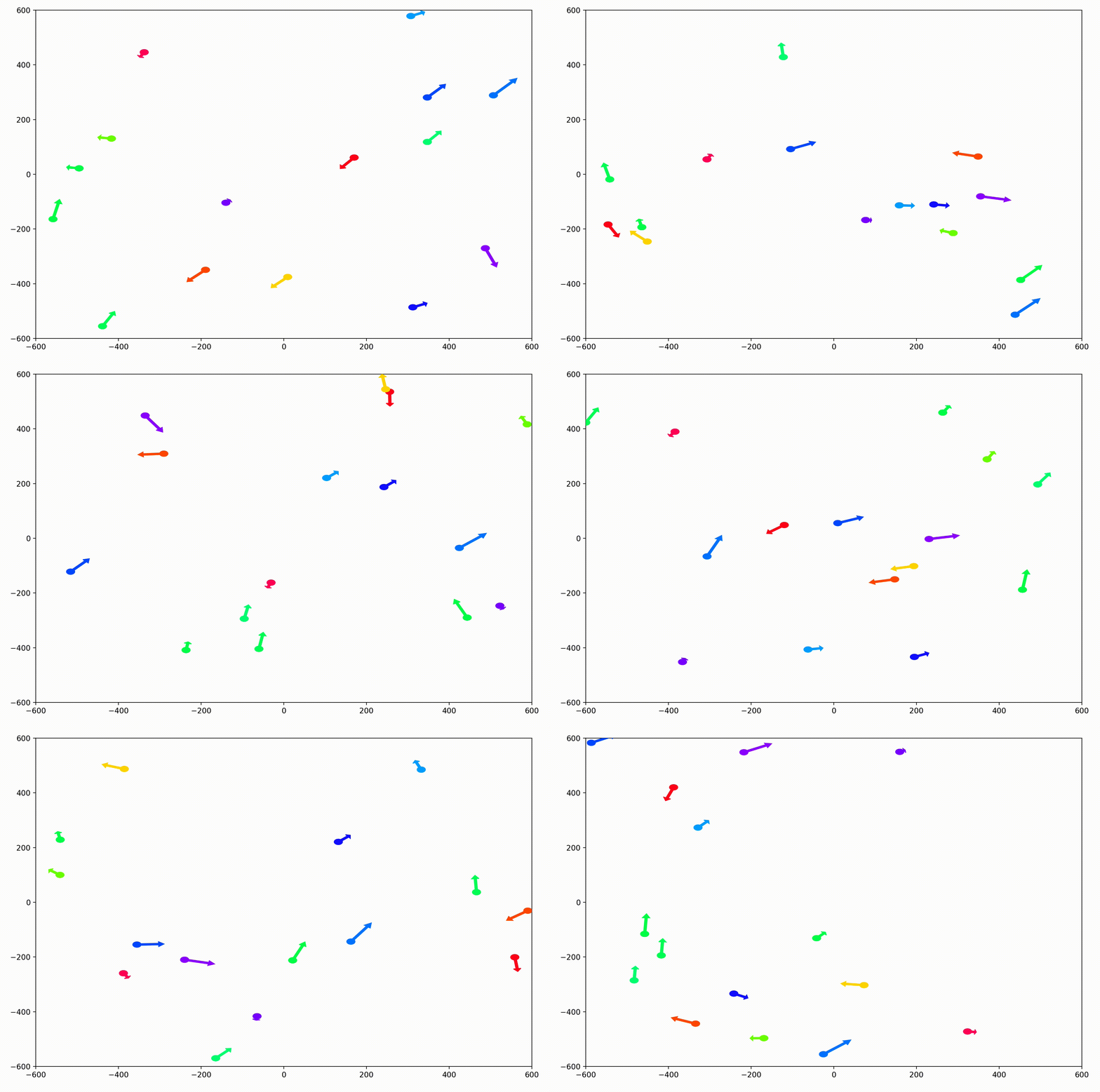
It’s okay if the behavior isn’t immediately obvious. It’s subtle. And if you think you predicted it correctly, great job!

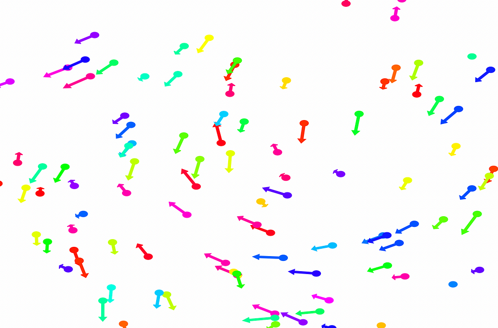
As it turned out, the agents didn’t organize themselves into herds by species very well at all. Instead, the only agents who seem to stick together are the ones who have both similar species and similar travel speed. You can see this happening most often with the slower green agents, the pair of blue agents, and the fast blue and purple agents shooting across the bottom of the screen. Notably, the agents seem to prioritize speed over species similarity when “choosing” who to travel with. You can see this most often with the light, dark blue, and even purple agents.

This makes perfect sense in the dynamics we defined, since each agent’s speed is constant, and agents with different speeds will ultimately fall behind or run away from their comrades. And yet, its somewhat surprising.

Fundamentally, this is because the behavior is emergent. In other words, we didn’t explicitly tell the agents to behave in this way as a group. Rather, they “derived” this behavior from the simple set of instructions, which we gave to each individual agent in an identical encoded format.

Visualization, Emergence, and Data Insights

We began this journey with the simple goal of visualizing an ABM to make sure on a high level that the dynamics we would set up would work as intended. But in addition to accomplishing this, we stumbled upon an emergent behavior which we may not have even considered when creating the model.

This illustrates an important partnership with respect to visualization in data science, simulations, and modeling across the board. Discovering emergent behavior in complex systems can be accelerated by new perspectives on the model or dataset. This isn’t only true for agent-based modeling. It applies to obtaining insights across the rest of data science as well. And creating new and creative visualizations provides a sure-fire way to get such perspectives.

If you’d like to play around with this model and visualization further, you can get the code at github.com/dreamchef/abm-viz. I’d love to hear what else you may find, or your thoughts on my work, in the comments! Feel free to reach out to me on Twitter and LinkedIn as well. Have a great day!

Unless otherwise noted, all images and animations were created by the author.

Visualizing Dynamical Behavior in Agent-Based Models was originally published in Towards Data Science on Medium, where people are continuing the conversation by highlighting and responding to this story.