

Improving LLM Inference Speeds on CPUs with Model Quantization
Discover how to significantly improve inference latency on CPUs using quantization techniques for mixed, int8, and int4 precisions
One of the most significant challenges the AI space faces is the need for computing resources to host large-scale production-grade LLM-based applications. At scale, LLM applications require redundancy, scalability, and reliability, which have historically been only possible on general computing platforms like CPUs. Still, the prevailing narrative today is that CPUs cannot handle LLM inference at latencies comparable with high-end GPUs.
One open-source tool in the ecosystem that can help address inference latency challenges on CPUs is the Intel Extension for PyTorch (IPEX), which provides up-to-date feature optimizations for an extra performance boost on Intel hardware. IPEX delivers a variety of easy-to-implement optimizations that make use of hardware-level instructions. This tutorial will dive into the theory of model compression and the out-of-the-box model compression techniques IPEX provides. These compression techniques directly impact LLM inference performance on general computing platforms, like Intel 4th and 5th-generation CPUs.
Inference Latency in Application Development
Second only to application safety and security, inference latency is one of the most critical parameters of an AI application in production. Regarding LLM-based applications, latency or throughput is often measured in tokens/second. As illustrated in the simplified inference processing sequence below, tokens are processed by the language model and then de-tokenized into natural language.
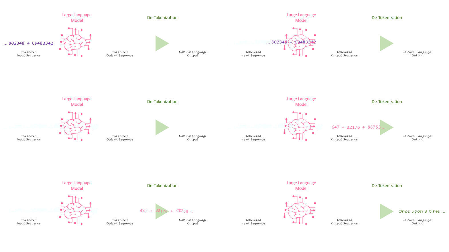
Interpreting inference this way can sometimes lead us astray because we analyze this component of AI applications in abstraction of the traditional production software paradigm. Yes, AI apps have their nuances, but at the end of the day, we are still talking about transactions per unit of time. If we start to think about inference as a transaction, like any other, from an application design point of view, the problem becomes less complex. For example, let’s say we have a chat application that has the following requirements:
- Average of 300 user sessions per hour
- Average of 5 transactions (LLM inference requests) per user per session
- Average 100 tokens generated per transaction
- Each session has an average of 10,000ms (10s) overhead for user authentication, guardrailing, network latency, and pre/post-processing.
- Users take an average of 30,000ms (30s) to respond when actively engaged with the chatbot.
- The average total active session time goal is 3 minutes or less.
Below, you can see that with some simple napkin math, we can get some approximate calculations for the required latency of our LLM inference engine.

Achieving required latency thresholds in production is a challenge, especially if you need to do it without incurring additional compute infrastructure costs. In the remainder of this article, we will explore one way that we can significantly improve inference latency through model compression.
Model Compression
Model compression is a loaded term because it addresses a variety of techniques, such as model quantization, distillation, pruning, and more. At their core, the chief aim of these techniques is to reduce the computational complexity of neural networks.
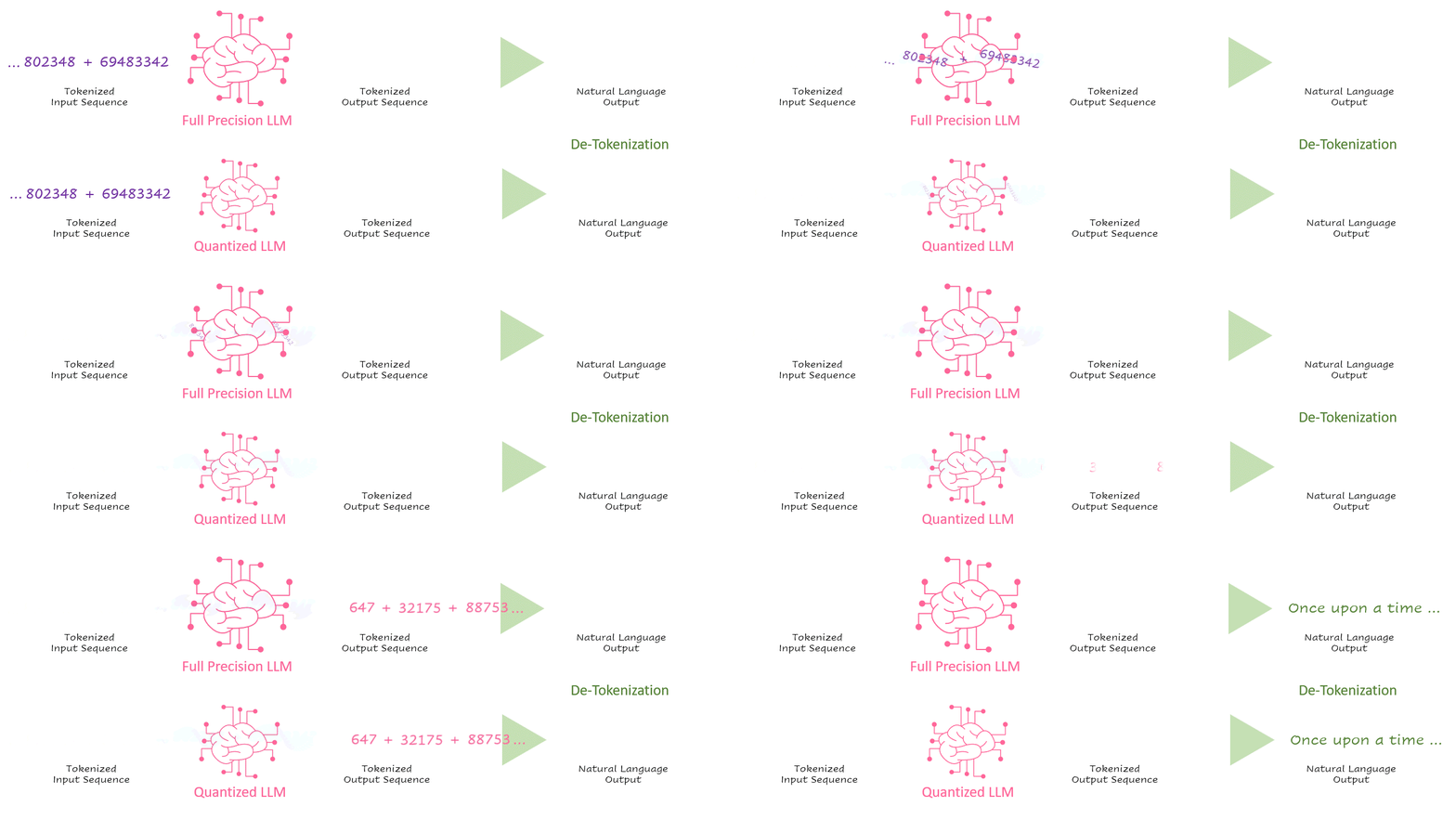
The method we will focus on today is model quantization, which involves reducing the byte precision of the weights and, at times, the activations, reducing the computational load of matrix operations and the memory burden of moving around larger, higher precision values. The figure below illustrates the process of quantifying fp32 weights to int8.

It is worth mentioning that the reduction of complexity by a factor of 4 that results from quantizing from fp32 (full precision) to int8 (quarter precision) does not result in a 4x latency reduction during inference because inference latency involves more factors beyond just model-centric properties.
Like with many things, there is no one-size-fits-all approach, and in this article, we will explore three of my favorite techniques for quantizing models using IPEX:
Mixed-Precision (bf16/fp32)
This technique quantizes some but not all of the weights in the neural network, resulting in a partial compression of the model. This technique is ideal for smaller models, like the <1B LLMs of the world.
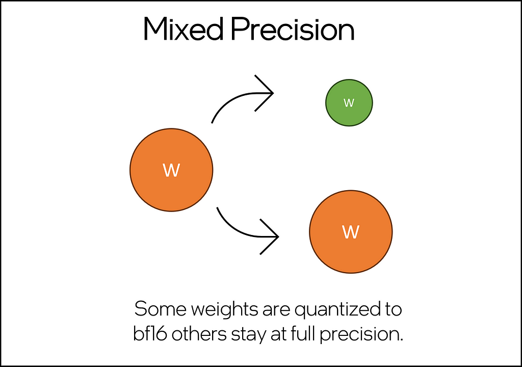
The implementation is quite straightforward: using hugging face transformers, a model can be loaded into memory and optimized using the IPEX llm-specific optimization function ipex.llm.optimize(model, dtype=dtype) by setting dtype = torch.bfloat16, we can activate the mixed precision inference capability, which improves the inference latency over full-precision (fp32) and stock.
import sys
import os
import torch
import intel_extension_for_pytorch as ipex
from transformers import AutoTokenizer, AutoModelForCausalLM, pipeline

# PART 1: Model and tokenizer loading using transformers
tokenizer = AutoTokenizer.from_pretrained("Intel/neural-chat-7b-v3-3")
model = AutoModelForCausalLM.from_pretrained("Intel/neural-chat-7b-v3-3")

# PART 2: Use IPEX to optimize the model
#dtype = torch.float # use for full precision FP32
dtype = torch.bfloat16 # use for mixed precision inference
model = ipex.llm.optimize(model, dtype=dtype)

# PART 3: Create a hugging face inference pipeline and generate results
pipe = pipeline("text-generation", model=model, tokenizer=tokenizer)
st = time.time()
results = pipe("A fisherman at sea...",  max_length=250)
end = time.time()
generation_latency = end-st

print('generation latency: ', generation_latency)
print(results[0]['generated_text'])
Of the three compression techniques we will explore, this is the easiest to implement (measured by unique lines of code) and offers the smallest net improvement over a non-quantized baseline.
SmoothQuant (int8)
This technique addresses the core challenges of quantizing LLMs, which include handling large-magnitude outliers in activation channels across all layers and tokens, a common issue that traditional quantization techniques struggle to manage effectively. This technique employs a joint mathematical transformation on both weights and activations within the model. The transformation strategically reduces the disparity between outlier and non-outlier values for activations, albeit at the cost of increasing this ratio for weights. This adjustment renders the Transformer layers “quantization-friendly,” enabling the successful application of int8 quantization without degrading model quality.
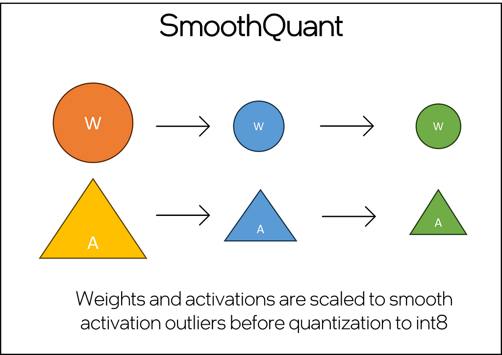
Below, you’ll find a simple SmoothQuant implementation — omitting the code for creating the DataLoader, which is a common and well-documented PyTorch principle. SmoothQuant is an accuracy-aware post-training quantization recipe, meaning that by providing a calibration dataset and model you will be able to provide a baseline and limit the language modeling degradation. The calibration model generates a quantization configuration, which is then passed to ipex.llm.optimize() along with the SmoothQuant mapping. Upon execution, the SmoothQuant is applied, and the model can be tested using the .generate() method.
import torch
import intel_extension_for_pytorch as ipex
from intel_extension_for_pytorch.quantization import prepare
import transformers

# PART 1: Load model and tokenizer from Hugging Face + Load SmoothQuant config mapping
tokenizer = AutoTokenizer.from_pretrained("Intel/neural-chat-7b-v3-3")
model = AutoModelForCausalLM.from_pretrained("Intel/neural-chat-7b-v3-3")
qconfig = ipex.quantization.get_smooth_quant_qconfig_mapping()

# PART 2: Configure calibration
# prepare your calibration dataset samples
calib_dataset = DataLoader({Your dataloader parameters})
example_inputs = # provide a sample input from your calib_dataset
calibration_model = ipex.llm.optimize(
  model.eval(),
  quantization_config=qconfig,
)
prepared_model = prepare(
  calibration_model.eval(), qconfig, example_inputs=example_inputs
)
with torch.no_grad():
  for calib_samples in enumerate(calib_dataset):
    prepared_model(calib_samples)
prepared_model.save_qconf_summary(qconf_summary=qconfig_summary_file_path)

# PART 3: Model Quantization using SmoothQuant
model = ipex.llm.optimize(
  model.eval(),
  quantization_config=qconfig,
  qconfig_summary_file=qconfig_summary_file_path,
)

# generation inference loop
with torch.inference_mode():
    model.generate({your generate parameters})
SmoothQuant is a powerful model compression technique and helps significantly improve inference latency over full-precision models. Still, it requires a little upfront work to prepare a calibration dataset and model.
Weight-Only Quantization (int8 and int4)
Compared to traditional int8 quantization applied to both activation and weight, weight-only quantization (WOQ) offers a better balance between performance and accuracy. It is worth noting that int4 WOQ requires dequantizing to bf16/fp16 before computation (Figure 4), which introduces an overhead in compute. A basic WOQ technique, tensor-wise asymmetric Round To Nearest (RTN) quantization, presents challenges and often leads to reduced accuracy (source). However, literature (Zhewei Yao, 2022) suggests that groupwise quantizing the model’s weights helps maintain accuracy. Since the weights are only dequantized for computation, a significant memory advantage remains despite this extra step.
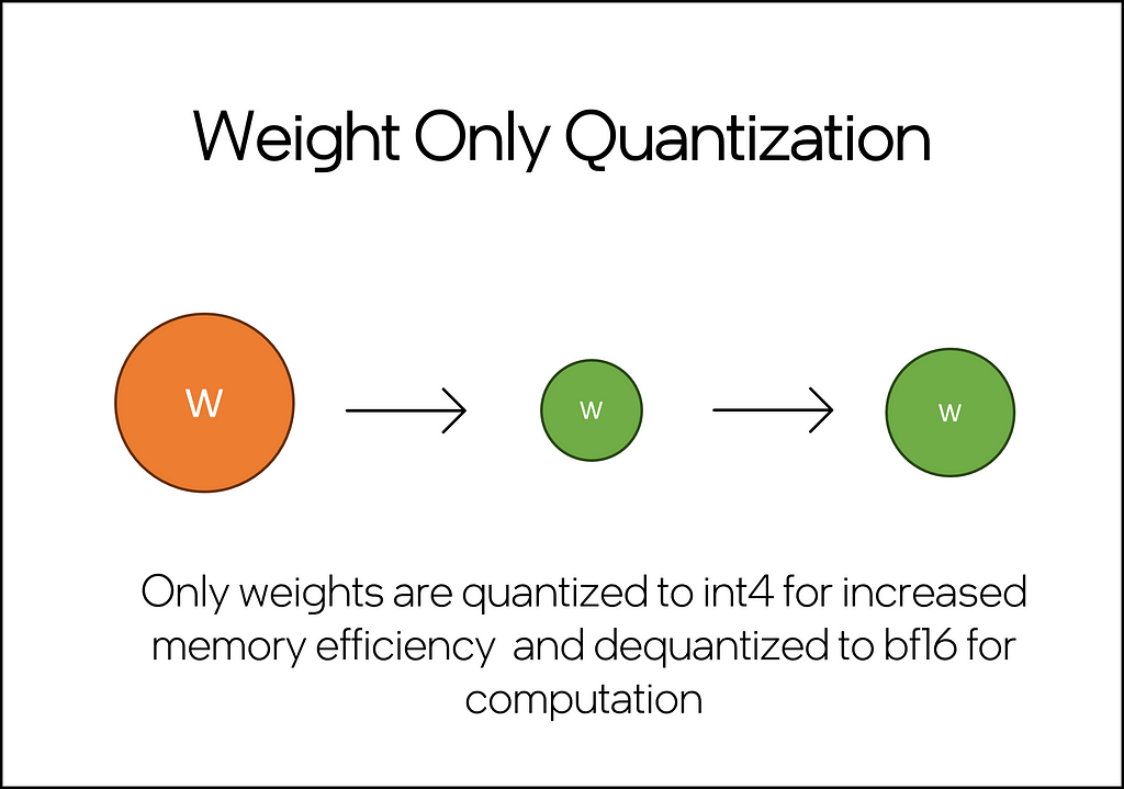
The WOQ implementation below showcases the few lines of code required to quantize a model from Hugging Face with this technique. As with the previous implementations, we start by loading a model and tokenizer from Hugging Face. We can use the get_weight_only_quant_qconfig_mapping() method to configure the WOQ recipe. The recipe is then passed to the ipex.llm.optimize() function along with the model for optimization and quantization. The quantized model can then be used for inference with the .generate() method.
import torch
import intel_extension_for_pytorch as ipex
import transformers

# PART 1: Model and tokenizer loading
tokenizer = AutoTokenizer.from_pretrained("Intel/neural-chat-7b-v3-3")
model = AutoModelForCausalLM.from_pretrained("Intel/neural-chat-7b-v3-3")

# PART 2: Preparation of quantization config
qconfig = ipex.quantization.get_weight_only_quant_qconfig_mapping(
  weight_dtype=torch.qint8, # or torch.quint4x2
  lowp_mode=ipex.quantization.WoqLowpMode.NONE, # or FP16, BF16, INT8
)
checkpoint = None # optionally load int4 or int8 checkpoint

# PART 3: Model optimization and quantization
model = ipex.llm.optimize(model, quantization_config=qconfig, low_precision_checkpoint=checkpoint)

# PART 4: Generation inference loop
with torch.inference_mode():
    model.generate({your generate parameters})
As you can see, WOQ provides a powerful way to compress models down to a fraction of their original size with limited impact on language modeling capabilities.
Conclusion and Discussion
As an engineer at Intel, I’ve worked closely with the IPEX engineering team at Intel. This has afforded me a unique insight into its advantages and development roadmap, making IPEX a preferred tool. However, for developers seeking simplicity without the need to manage an extra dependency, PyTorch offers three quantization recipes: Eager Mode, FX Graph Mode (under maintenance), and PyTorch 2 Export Quantization, providing strong, less specialized alternatives.
No matter what technique you choose, model compression techniques will result in some degree of language modeling performance loss, albeit in <1% in many cases. For this reason, it’s essential to evaluate the application’s fault tolerance and establish a baseline for model performance at full (FP32) and/or half-precision (BF16/FP16) before pursuing quantization.
In applications that leverage some degree of in-context learning, like Retrieval Augmented Generation (RAG), model compression might be an excellent choice. In these cases, the mission-critical knowledge is spoon-fed to the model at the time of inference, so the risk is heavily reduced even with low-fault-tolerant applications.
Quantization is an excellent way to address LLM inference latency concerns without upgrading or expanding compute infrastructure. It is worth exploring regardless of your use case, and IPEX provides a good option to start with just a few lines of code.
A few exciting things to try would be:
- Test the sample code in this tutorial on the Intel Developer Cloud’s free Jupyter Environment.
- Take an existing model that you’re running on an accelerator at complete precision and test it out on a CPU at int4/int8
- Explore all three techniques and determine which works best for your use case. Make sure to compare the loss of language modeling performance, not just latency.
- Upload your quantized model to the Hugging Face Model Hub! If you do, let me know — I’d love to check it out!
Thank you for reading! Don’t forget to follow my profile for more articles like this!
Improving LLM Inference Latency on CPUs with Model Quantization was originally published in Towards Data Science on Medium, where people are continuing the conversation by highlighting and responding to this story.
Originally appeared here:
Improving LLM Inference Latency on CPUs with Model Quantization
Go Here to Read this Fast! Improving LLM Inference Latency on CPUs with Model Quantization
