3 Key Encoding Techniques for Machine Learning: A Beginner-Friendly Guide

3 Key Encoding Techniques for Machine Learning: A Beginner-Friendly Guide with Pros, Cons, and Python Code Examples

How should we choose between label, one-hot, and target encoding?

Why Do We Need Encoding?
In the realm of machine learning, most algorithms demand inputs in numeric form, especially in many popular Python frameworks. For instance, in scikit-learn, linear regression, and neural networks require numerical variables. This means we need to transform categorical variables into numeric ones for these models to understand them. However, this step isn’t always necessary for models like tree-based ones.

Today, I’m thrilled to introduce three fundamental encoding techniques that are essential for every budding data scientist! Plus, I’ve included a practical tip to help you see these techniques in action at the end! Unless stated, all the codes and pictures are created by the author.

Label Encoding / Ordinal Encoding
Both label encoding and ordinal encoding involve assigning integers to different classes. The distinction lies in whether the categorical variable inherently has an order. For example, responses like ‘strongly agree,’ ‘agree,’ ‘neutral,’ ‘disagree,’ and ‘strongly disagree’ are ordinal as they follow a specific sequence. When a variable doesn’t have such an order, we use label encoding.

Let’s delve into label encoding.
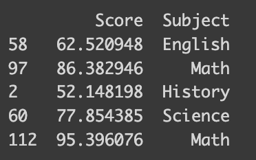
I’ve prepared a synthetic dataset with math test scores and students’ favorite subjects. This dataset is designed to reflect higher scores for students who prefer STEM subjects. The following code shows how it is synthesized.

import numpy as np
import pandas as pd

math_score = [60, 70, 80, 90]
favorite_subject = ["History", "English", "Science", "Math"]
std_deviation =  5  
num_samples = 30   

# Generate 30 samples with a normal distribution
scores = []
subjects = []
for i in range(4):
  scores.extend(np.random.normal(math_score[i], std_deviation, num_samples))
  subjects.extend([favorite_subject[i]]*num_samples)

data = {'Score': scores, 'Subject': subjects}
df_math = pd.DataFrame(data)

# Print the DataFrame
print(df_math.sample(frac=0.04))import numpy as np
import pandas as pd
import random

math_score = [60, 70, 80, 90]
favorite_subject = ["History", "English", "Science", "Math"]
std_deviation =  5  # Standard deviation in cm
num_samples = 30   # Number of samples

# Generate 30 samples with a normal distribution
scores = []
subjects = []
for i in range(4):
  scores.extend(np.random.normal(math_score[i], std_deviation, num_samples))
  subjects.extend([favorite_subject[i]]*num_samples)

data = {'Score': scores, 'Subject': subjects}
df_math = pd.DataFrame(data)

# Print the DataFrame
sampled_index = random.sample(range(len(df_math)), 5)
sampled = df_math.iloc[sampled_index]
print(sampled)

You’ll be amazed at how simple it is to encode your data — it takes just a single line of code! You can pass a dictionary that maps between the subject name and number to the default method of the pandas dataframe like the following.

# Simple way
df_math['Subject_num'] = df_math['Subject'].replace({'History': 0, 'Science': 1, 'English': 2, 'Math': 3})
print(df_math.iloc[sampled_index])

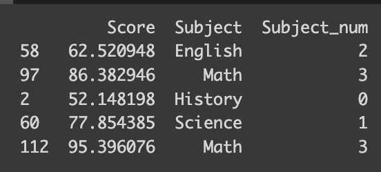
But what if you’re dealing with a vast array of classes, or perhaps you’re looking for a more straightforward approach? That’s where the scikit-learn library’s `LabelEncoder` function comes in handy. It automatically encodes your classes based on their alphabetical order. For the best experience, I recommend using version 1.4.0, which supports all the encoders we’re discussing.

# Scikit-learn
from sklearn.preprocessing import LabelEncoder
le = LabelEncoder()
df_math["Subject_num_scikit"] = le.fit_transform(df_math[['Subject']])
print(df_math.iloc[sampled_index])

However, there’s a catch. Consider this: our dataset doesn’t imply an ordinal relationship between favorite subjects. For instance, ‘History’ is encoded as 0, but that doesn’t mean it’s ‘inferior’ to ‘Math,’ which is encoded as 3. Similarly, the numerical gap between ‘English’ and ‘Science’ is smaller than that between ‘English’ and ‘History,’ but this doesn’t necessarily reflect their relative similarity.

This encoding approach also affects interpretability in some algorithms. For example, in linear regression, each coefficient indicates the expected change in the outcome variable for a one-unit change in a predictor. But how do we interpret a ‘unit change’ in a subject that’s been numerically encoded? Let’s put this into perspective with a linear regression on our dataset.

from sklearn.linear_model import LinearRegression

model = LinearRegression()
model.fit(df_math[["Subject_num"]], df_math[["Score"]])

coefficients = model.coef_

print("Coefficients:", coefficients)

How can we interpret the coefficient 8.26 here? The naive way would be when the label changes by 1 unit, the test score changes by 8. However, it is not really true from Science (encoded as 1) to History (encoded as 2) since I synthesized in a way that the mean score would be 80 and 70 respectively. So, we should not interpret the coefficient when there is no meaning in the way we label each class!

Now, moving on to ordinal encoding, let’s apply it to another synthetic dataset, this time focusing on height and school categories. I’ve tailored this dataset to reflect average heights for different school levels: 110 cm for kindergarten, 140 cm for elementary school, and so on. Let’s see how this plays out.

import numpy as np
import pandas as pd

# Set the parameters
mean_height = [110, 140, 160, 175, 180]  # Mean height in cm
grade = ["kindergarten", "elementary school", "middle school", "high school", "college"]
std_deviation = 5  # Standard deviation in cm
num_samples = 10   # Number of samples

# Generate 10 samples with a normal distribution
heights = []
grades = []
for i in range(5):
  heights.extend(np.random.normal(mean_height[i], std_deviation, num_samples))
  grades.extend([grade[i]]*10)

data = {'Grade': grades, 'Height': heights}
df = pd.DataFrame(data)

sampled_index = random.sample(range(len(df)), 5)
sampled = df.iloc[sampled_index]
print(sampled)

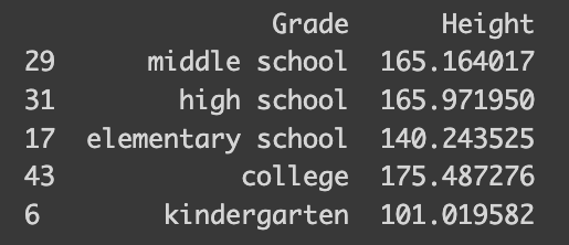
The `OrdinalEncoder` from scikit-learn’s preprocessing toolkit is a real gem for handling ordinal variables. It’s intuitive, automatically determining the ordinal structure and encoding it accordingly. If you look at encoder.categories_, you can check how the variable was encoded.

from sklearn.preprocessing import OrdinalEncoder

encoder = OrdinalEncoder(categories=[grade])
df['Category'] = encoder.fit_transform(df[['Grade']])
print(encoder.categories_)
print(df.iloc[sampled_index])

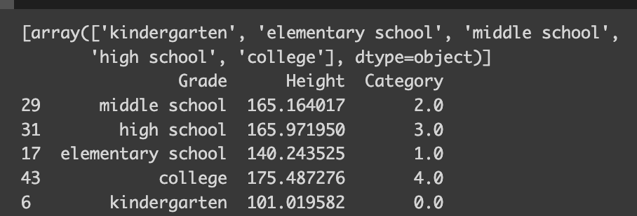
When it comes to ordinal categorical variables, interpreting linear regression models becomes more straightforward. The encoding reflects the degree of education in a numerical order — the higher the education level, the higher its corresponding value.

from sklearn.linear_model import LinearRegression

model = LinearRegression()
model.fit(df[["Category"]], df[["Height"]])

coefficients = model.coef_

print("Coefficients:", coefficients)

height_diff = [mean_height[i] - mean_height[i-1] for i in range(1, len(mean_height),1)]
print("Average Height Difference:", sum(height_diff)/len(height_diff))

The model reveals something quite intuitive: a one-unit change in school type corresponds to a 17.5 cm increase in height. This makes perfect sense given our dataset!

So, let’s wrap up with a quick summary of label/ordinal encoding:

Pros:
– Simplicity: It’s user-friendly and easy to implement.
– Efficiency: This method is light on computational resources and memory, creating just one new numerical feature.
– Ideal for Ordinal Categories: It shines when dealing with categorical variables that have a natural order.

Cons:
– Implied Order: One potential downside is that it can introduce a sense of order where none exists, potentially leading to misinterpretation (like assuming a category labeled ‘3’ is superior to one labeled ‘2’).
– Not Always Suitable: Certain algorithms, such as linear or logistic regression, might incorrectly interpret the encoded numerical values as having ordinal significance.

One-hot encoding

Next up, let’s dive into another encoding technique that addresses the interpretability issue: One-hot encoding.

The core issue with label encoding is that it imposes an ordinal structure on variables that don’t inherently have one, by replacing categories with numerical values. One-hot encoding tackles this by creating a separate column for each class. Each of these columns contains binary values, indicating whether the row belongs to that class. It’s like pivoting the data to a wider format, for those who are familiar with that concept. To make this clearer, let’s see an example using the math_score and subject data. The `OneHotEncoder` from sklearn.preprocessing is perfect for this task.

from sklearn.preprocessing import OneHotEncoder

data = {'Score': scores, 'Subject': subjects}
df_math = pd.DataFrame(data)

y = df_math["Score"] # Target 
x = df_math.drop('Score', axis=1)

# Define encoder
encoder = OneHotEncoder()
x_ohe = encoder.fit_transform(x)
print("Type:",type(x_ohe))
# Convert x_ohe to array so that it is more compatible
x_ohe = x_ohe.toarray()
print("Dimension:", x_ohe.shape)

# Convet back to pandas dataframe
x_ohe = pd.DataFrame(x_ohe, columns=encoder.get_feature_names_out())
df_math_ohe = pd.concat([y, x_ohe], axis=1)
sampled_ohe_idx = random.sample(range(len(df_math_ohe)), 5)
print(df_math_ohe.iloc[sampled_ohe_idx])

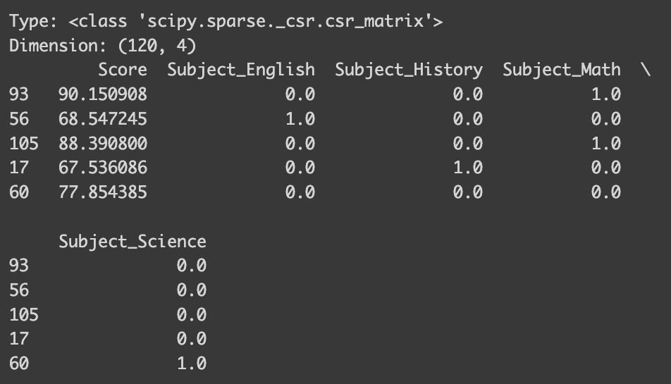
Now, instead of having a single ‘Subject’ column, our dataset features individual columns for each subject. This effectively eliminates any unintended ordinal structure! However, the process here is a bit more involved, so let me explain.

Like with label/ordinal encoding, you first need to define your encoder. But the output of one-hot encoding differs: while label/ordinal encoding returns a numpy array, one-hot encoding typically produces a `scipy.sparse._csr.csr_matrix`. To integrate this with a pandas dataframe, you’ll need to convert it into an array. Then, create a new dataframe with this array and assign column names, which you can get from the encoder’s `get_feature_names_out()` method. Alternatively, you can get numpy array directly by setting `sparse_output=False` when defining the encoder.

However, in practical applications, you don’t need to go through all these steps. I’ll show you a more streamlined approach using `make_column_transformer` towards the end of our discussion!

Now, let’s proceed with running a linear regression on our one-hot encoded data. This should make the interpretation much easier, right?

model = LinearRegression()
model.fit(x_ohe, y)

coefficients = model.coef_
intercept = model.intercept_

print("Coefficients:", coefficients)
print(encoder.get_feature_names_out())
print("Intercept:",intercept)

But wait, why are the coefficients so tiny, and the intercept so large? What’s going wrong here? This conundrum is a specific issue in linear regression known as perfect multicollinearity. Perfect multicollinearity occurs when when one variable in a linear regression model can be perfectly predicted from the others, which in the case of one-hot encoding happens because one class can be inferred if all other classes are zero. To sidestep this problem, we can drop one of the classes by setting `OneHotEncoder(drop=”first”)`. Let’s check out the impact of this adjustment.

encoder_with_drop = OneHotEncoder(drop="first")
x_ohe_drop = encoder_with_drop.fit_transform(x)

# if you don't sparse_output = False, you need to run the following to convert type
x_ohe_drop = x_ohe_drop.toarray()

x_ohe_drop = pd.DataFrame(x_ohe_drop, columns=encoder_with_drop.get_feature_names_out())

model = LinearRegression()
model.fit(x_ohe_drop, y)

coefficients = model.coef_
intercept = model.intercept_

print("Coefficients:", coefficients)
print(encoder_with_drop.get_feature_names_out())
print("Intercept:",intercept)

Here, the column for English has been dropped, and now the coefficients seem much more reasonable! Plus, they’re easier to interpret. When all the one-hot encoded columns are zero (indicating English as the favorite subject), we predict the test score to be around 71 (aligned with our defined average score for English). For History, it would be 71 minus 11 equals 60, for Math, 71 plus 19, and so on.

However, there’s a significant caveat with one-hot encoding: it can lead to high-dimensional datasets, especially when the variable has a large number of classes. Let’s consider a dataset that includes 1000 rows, each representing a unique product with various features, including a category that spans 100 different types.

# Define 1000 categories (for simplicity, these are just numbered)
categories = [f"Category_{i}" for i in range(1, 200)]

manufacturers = ["Manufacturer_A", "Manufacturer_B", "Manufacturer_C"]
satisfied = ["Satisfied", "Not Satisfied"]
n_rows = 1000  

# Generate random data
data = {
    "Product_ID": [f"Product_{i}" for i in range(n_rows)],
    "Category": [random.choice(categories) for _ in range(n_rows)],
    "Price": [round(random.uniform(10, 500), 2) for _ in range(n_rows)],
    "Quality": [random.choice(satisfied) for _ in range(n_rows)],
    "Manufacturer": [random.choice(manufacturers) for _ in range(n_rows)],
}

df = pd.DataFrame(data)

print("Dimension before one-hot encoding:",df.shape)
print(df.head())

Note that the dataset’s dimensions are 1000 rows by 5 columns. Now, let’s observe the changes after applying a one-hot encoder.

# Now do one-hot encoding
encoder = OneHotEncoder(sparse_output=False)

# Reshape the 'Category' column to a 2D array as required by the OneHotEncoder
category_array = df['Category'].values.reshape(-1, 1)

one_hot_encoded_array = encoder.fit_transform(category_array)
one_hot_encoded_df = pd.DataFrame(one_hot_encoded_array, columns=encoder.get_feature_names_out(['Category']))
encoded_df = pd.concat([df.drop('Category', axis=1), one_hot_encoded_df], axis=1)

print("Dimension after one-hot encoding:", encoded_df.shape)

After applying one-hot encoding, our dataset’s dimension balloons to 1000×201 — a whopping 40 times larger than before. This increase is a concern, as it demands more memory. Moreover, you’ll notice that most of the values in the newly created columns are zeros, resulting in what we call a sparse dataset. Certain models, especially tree-based ones, struggle with sparse data. Furthermore, other challenges arise when dealing with high-dimensional data often referred to as the ‘curse of dimensionality.’ Also, since one-hot encoding treats each class as an individual column, we lose any ordinal information. Therefore, if the classes in your variable inherently have a hierarchical order, one-hot encoding might not be your best choice.

How do we tackle these disadvantages? One approach is to use a different encoding method. Alternatively, you can limit the number of classes in the variable. Often, even with a large number of classes, the majority of values for a variable are concentrated in just a few classes. In such cases, treating these minority classes as ‘others’ can be effective. This can be achieved by setting parameters like `min_frequency` or `max_categories` in OneHotEncoder. Another strategy for dealing with sparse data involves techniques like feature hashing, which essentially simplifies the representation by mapping multiple categories to a lower-dimensional space using a hash function, or dimension reduction techniques like PCA.

Here’s a quick summary of One-hot encoding:

Pros:
– Prevents Misleading Interpretations: It avoids the risk of models misinterpreting the data as having some sort of order, an issue prevalent in label/target encoding.
– Suitable for Non-Ordinal Features: Ideal for categorical data without an ordinal relationship.

Cons:
– Dimensionality Increase: Leads to a significant increase in the dataset’s dimensionality, which can be problematic, especially for variables with many categories.
– Sparse Matrix: Results in many columns filled with zeros, creating sparse data.
– Not Efficient with High Cardinality Features: Less effective for variables with a large number of categories.

Target Encoding
Let’s now explore target encoding, a technique particularly effective with high-cardinality data and in models like tree-based algorithms.

The essence of target encoding is to leverage the information from the value of the dependent variable. Its implementation varies depending on the task. In regression, we encode the target variable by the mean of the dependent variable for each class. For binary classification, it’s done by encoding the target variable with the probability of being in one class (calculated as the number of rows in that class where the outcome is 1, divided by the total number of rows in the class). In multiclass classification, the categorical variable is encoded based on the probability of belonging to each class, resulting in as many new columns as there are classes in the dependent variable. To clarify, let’s use the same product dataset we employed for one-hot encoding.

Let’s begin with target encoding for a regression task. Imagine we want to predict the price of goods and aim to encode the product type. Similar to other encodings, we use TargetEncoder from sklearn.preprocessing!

from sklearn.preprocessing import TargetEncoder
x = df.drop(["Price"], axis=1)
x_need_encode = df["Category"].to_frame()
y = df["Price"]

# Define encoder
encoder = TargetEncoder()
x_encoded = encoder.fit_transform(x_need_encode, y)

# Encoder with 0 smoothing
encoder_no_smooth = TargetEncoder(smooth=0)
x_encoded_no_smooth = encoder_no_smooth.fit_transform(x_need_encode, y)

x_encoded = pd.DataFrame(x_encoded, columns=["encoded_category"])
data_target = pd.concat([x, x_encoded], axis=1)

print("Dimension before encoding:", df.shape)
print("Dimension after encoding:", data_target.shape)
print("---------")
print("Encoding")
print(encoder.encodings_[0][:5])
print(encoder.categories_[0][:5])
print(" ")
print("Encoding with no smooth")
print(encoder_no_smooth.encodings_[0][:5])
print(encoder_no_smooth.categories_[0][:5])
print("---------")
print("Mean by Category")
print(df.groupby("Category").mean("Price").head())
print("---------")
print("dataset:")
print(data_target.head())

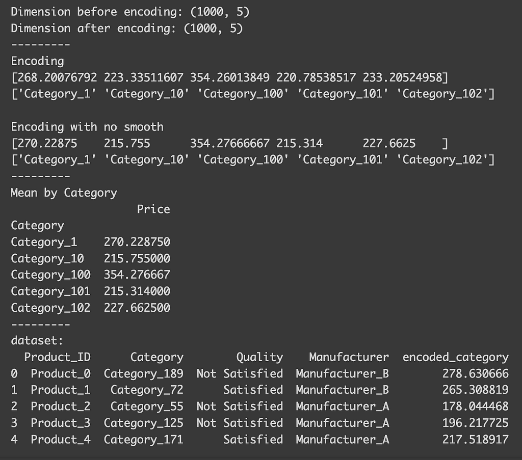
After the encoding, you’ll notice that, despite the variable having many classes, the dataset’s dimension remains unchanged (1000 x 5). You can also observe how each class is encoded. Although I mentioned that the encoding for each class is based on the mean of the target variable for that class, you’ll find that the actual mean differs slightly from the encoding using the default settings. This discrepancy arises because, by default, the function automatically selects a smoothing parameter. This parameter blends the local category mean with the overall global mean, which is particularly useful to prevent overfitting in categories with limited samples. If we set `smooth=0`, the encoded values align precisely with the actual means.

Now, let’s consider binary classification. Imagine our goal is to classify whether the quality of a product is satisfactory. In this scenario, the encoded value represents the probability of a category being ‘satisfactory.’

x = df.drop(["Quality"], axis=1)
x_need_encode = df["Category"].to_frame()
y = df["Quality"]

# Define encoder
encoder = TargetEncoder()
x_encoded = encoder.fit_transform(x_need_encode, y)


x_encoded = pd.DataFrame(x_encoded, columns=["encoded_category"])
data_target = pd.concat([x, x_encoded], axis=1)

print("Dimension:", data_target.shape)
print("---------")
print("Encoding")
print(encoder.encodings_[0][:5])
print(encoder.categories_[0][:5])
print("---------")
print(encoder.classes_)
print("---------")
print("dataset:")
print(data_target.head())

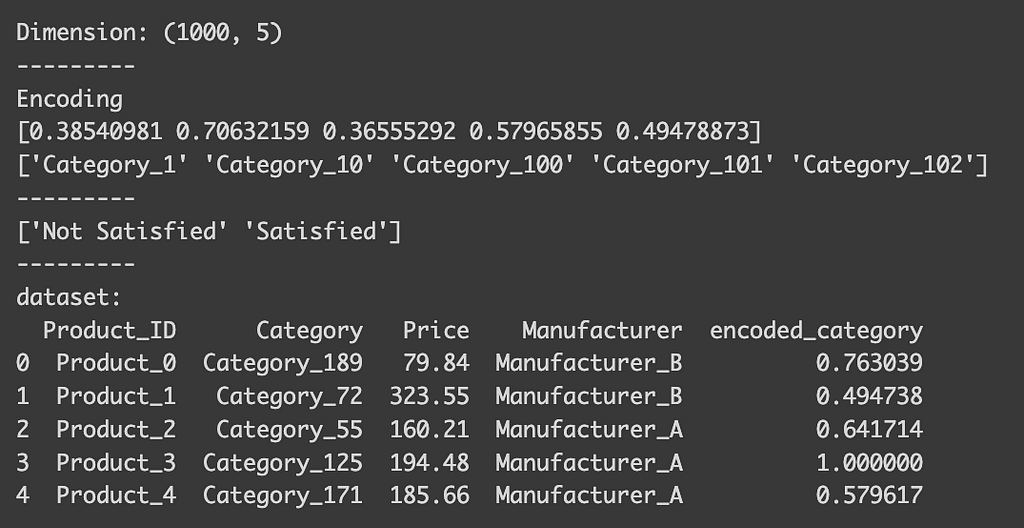
You can indeed see that the encoded_category represent the probability being “Satisfied” (float value between 0 and 1). To see how each class is encoded, you can check the `classes_` attribute of the encoder. For binary classification, the first value in the list is typically dropped, meaning that the column here indicates the probability of being satisfied. Conveniently, the encoder automatically detects the type of task, so there’s no need to specify that it’s a binary classification.

Lastly, let’s see multi-class classification example. Suppose we’re predicting which manufacturer produced a product.

x = df.drop(["Manufacturer"], axis=1)
x_need_encode = df["Category"].to_frame()
y = df["Manufacturer"]

# Define encoder
encoder = TargetEncoder()
x_encoded = encoder.fit_transform(x_need_encode, y)


x_encoded = pd.DataFrame(x_encoded, columns=encoder.classes_)
data_target = pd.concat([x, x_encoded], axis=1)

print("Dimension:", data_target.shape)
print("---------")
print("Encoding")
print(encoder.encodings_[0][:5])
print(encoder.categories_[0][:5])
print("---------")
print("dataset:")
print(data_target.head())

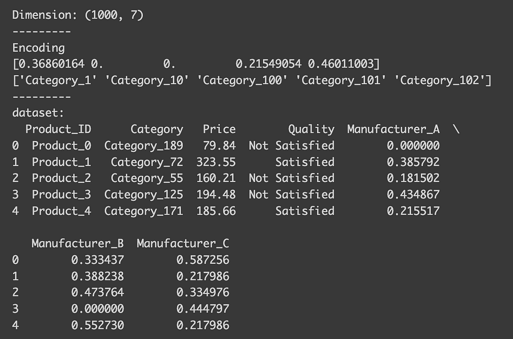
After encoding, you’ll see that we now have columns for each manufacturer. These columns indicate the probability of a product belonging to a certain category being produced by that manufacturer. Although our dataset has expanded slightly, the number of classes for the dependent variable is usually much smaller, so it’s unlikely to cause issues.

Target encoding is particularly advantageous for tree-based models. These models make splits based on feature values that most effectively separate the target variable. By directly incorporating the mean of the target variable, target encoding provides a clear and efficient means for the model to make these splits, often more so than other encoding methods.

However, caution is needed with target encoding. If there are only a few observations for a class, and these don’t represent the true mean for that class, there’s a risk of overfitting.

This leads to another crucial point: it’s vital to perform target encoding after splitting your data into training and testing sets. Doing it beforehand can lead to data leakage, as the encoding would be influenced by the outcomes in the test dataset. This could result in the model performing exceptionally well on the training dataset, giving you a false impression of its efficacy. Therefore, to accurately assess your model’s performance, ensure target encoding is done post train-test split.

Here’s a quick summary of target encoding:

Pros:
– Keeps Cardinality in Check: It’s highly effective for high cardinality features as it doesn’t increase the feature space.
– Can Capture Information Within Labels: By incorporating target data, it often enhances predictive performance.
– Useful for Tree-Based Models: Particularly advantageous for complex models such as random forests or gradient boosting machines.

Cons:
– Risk of Overfitting: There’s a heightened risk of overfitting, especially when categories have a limited number of observations.
– Target Leakage: It may inadvertently introduce future information into the model, i.e., details from the target variable that wouldn’t be accessible during actual predictions.
– Less Interpretable: Since the transformations are based on the target, they can be more challenging to interpret compared to methods like one-hot or label encoding.

Final tip
To wrap up, I’d like to offer some practical tips. Throughout this discussion, we’ve looked at different encoding techniques, but in reality, you might want to apply various encodings to different variables within a dataset. This is where `make_column_transformer` from sklearn.compose comes in handy. For example, suppose you’re predicting product prices and decide to use target encoding for the ‘Category’ due to its high cardinality, while applying one-hot encoding for ‘Manufacturer’ and ‘Quality’. To do this, you would define arrays containing the names of the variables for each encoding type and apply the function as shown below. This approach allows you to handle the transformed data seamlessly, leading you to an efficiently encoded dataset ready for your analyses!

from sklearn.compose import make_column_transformer
ohe_cols = ["Manufacturer"]
te_cols = ["Category", "Quality"]

encoding = make_column_transformer(
    (OneHotEncoder(), ohe_cols),
    (TargetEncoder(), te_cols)
)

x = df.drop(["Price"], axis=1)
y = df["Price"]

# Fit the transformer
x_encoded = encoding.fit_transform(x, y)
x_encoded = pd.DataFrame(x_encoded, columns=encoding.get_feature_names_out())

x_rest = x.drop(ohe_cols+te_cols, axis=1)
print(pd.concat([x_rest, x_encoded],axis=1).head()) 

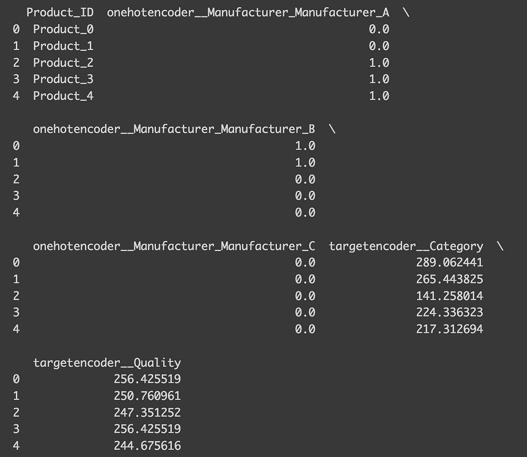
Thank you so much for taking the time to read through this! When I first embarked on my machine learning journey, choosing the right encoding techniques and understanding their implementation was quite a maze for me. I genuinely hope this article has shed some light for you and made your path a bit clearer!

Source:
Scikit-learn: Machine Learning in Python, Pedregosa et al., JMLR 12, pp. 2825–2830, 2011.
Documentation of Scikit-learn:
Ordinal encoder: https://scikit-learn.org/stable/modules/generated/sklearn.preprocessing.OrdinalEncoder.html#sklearn.preprocessing.OrdinalEncoder
Target encoder: https://scikit-learn.org/stable/modules/generated/sklearn.preprocessing.TargetEncoder.html#sklearn.preprocessing.TargetEncoder
One-hot encoder https://scikit-learn.org/stable/modules/generated/sklearn.preprocessing.OneHotEncoder.html#sklearn.preprocessing.OneHotEncoder

3 Key Encoding Techniques for Machine Learning: A Beginner-Friendly Guide was originally published in Towards Data Science on Medium, where people are continuing the conversation by highlighting and responding to this story.