Year: 2024

Implementing a simple neural network framework from scratch

Despite doing some work and research in the AI ecosystem for some time, I didn’t truly stop to think about backpropagation and gradient updates within neural networks until recently. This article seeks to rectify that and will hopefully provide a thorough yet easy-to-follow dive into the topic by implementing a simple (yet somewhat powerful) neural network framework from scratch.

Elementary Operations — The Network’s Core

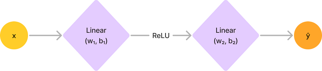
Fundamentally, a neural network is just a mathematical function from our input space to our desired output space. In fact, we can effectively “unwrap” any neural network into a function. Consider, for instance, the following simple neural network with two layers and one input:

We can now construct an equivalent function by going forwards layer by layer, starting from the input. Let’s follow our final function layer by layer:

1. At the input, we start with the identity function pred(x) = x
2. At the first linear layer, we get pred(x) = w₁x + b₁
3. The ReLU nets us pred(x) = max(0, w₁x + b₁)
4. At the final layer, we get pred(x) = w₂(max(0, w₁x + b₁)) + b₂

With more complicated nets, these functions of course get unwieldy, but the point is that we can construct such representations of neural networks.

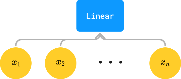
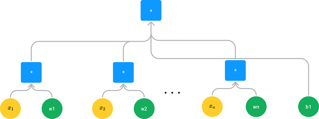
We can go one step further though — functions of this form are not extremely convenient for computation, but we can parse them into a more useful form, namely a syntax tree. For our simple net, the tree would look like this:

In this tree form, our leaves are parameters, constants, and inputs, and the other nodes are elementary operations whose arguments are their children. Of course, these elementary operations don’t have to be binary — the sigmoid operation, for instance, is unary (and so is ReLU if we don’t represent it as a max of 0 and x), and we can choose to support multiplication and addition of more than one input.

By thinking of our network as a tree of these elementary operations, we can now do a lot of things very easily with recursion, which will form the basis of both our backpropagation and forward propagation algorithms. In code, we can define a recursive neural network class that looks like this:

from dataclasses import dataclass, field
from typing import List

@dataclass
class NeuralNetNode:
    """A node in our neural network tree"""
    children: List['NeuralNetNode'] = field(default_factory=list)
    
    def op(self, x: List[float]) -> float:
        """The operation that this node performs"""
        raise NotImplementedError
    
    def forward(self) -> float:
        """Evaluate this node on the given input"""
        return self.op([child.forward() for child in self.children])
    
    # This is just for convenience
    def __call__(self) -> List[float]:
        return self.forward()

    def __repr__(self):
        return f'{self.__class__.__name__}({self.children})'

Going Backwards — Recursive Chain Rule

Suppose now that we have a differentiable loss function for our neural network, say MSE. Recall that MSE (for one sample) is defined as follows:

We now wish to update our parameters (the green circles in our tree representation) given the value of our loss. To do this, we need the derivative of our loss function with respect to each parameter. Calculating this directly from the loss is extremely difficult though — after all, our MSE is calculated in terms of the value predicted by our neural net, which can be an extraordinarily complicated function.

This is where very useful piece of mathematics — the chain rule — comes into play. Instead of being forced to compute our highly complex derivatives from the get-go, we can instead compute a series of simpler derivatives.

It turns out that the chain rule meshes very well with our recursive tree structure. The idea basically works as follows: assuming that we have simple enough elementary operations, each elementary operation knows its derivative with respect to all of its arguments. Given the derivative from the parent operation, we can thus compute the derivative of each child operation with respect to the loss function through simple multiplication. For a simple linear regression model using MSE, we can diagram it as follows:

Of course, some of our nodes don’t do anything with their derivatives — namely, only our leaf nodes care. But now each node can get the derivative of its output with respect to the loss function through this recursive process. We can thus add the following methods to our NeuralNetNode class:

def grad(self) -> List[float]:
    """The gradient of this node with respect to its inputs"""
    raise NotImplementedError
    
def backward(self, derivative_from_parent: float):
    """Propagate the derivative from the parent to the children"""
    self.on_backward(derivative_from_parent)
    deriv_wrt_children = self.grad()
    for child, derivative_wrt_child in zip(self.children, deriv_wrt_children):
        child.backward(derivative_from_parent * derivative_wrt_child)
        
def on_backward(self, derivative_from_parent: float):
    """Hook for subclasses to override. Things like updating parameters"""
    pass

Exercise 1: Try creating one of these trees for a simple linear regression model and perform the recursive gradient updates by hand for a couple of steps.

Note: For simplicity’s sake, we require our nodes to have only one parent (or none at all). If each node is allowed to have multiple parents, our backwards() algorithm becomes somewhat more complicated as each child needs to sum the derivative of its parents to compute its own. We can do this iteratively with a topological sort (e.g. see here) or still recursively, i.e. with reverse accumulation (though in this case we would need to do a second pass to actually update all of the parameters). This isn’t extraordinarily difficult, so I’ll leave it as an exercise to the reader (and will talk about it more in part 2, stay tuned).

Finishing Our Framework

Building Models

The rest of our code really just involves implementing parameters, inputs, and operations, and of course running our training. Parameters and inputs are fairly simple constructs:

import random

@dataclass
class Input(NeuralNetNode):
    """A leaf node that represents an input to the network"""
    value: float=0.0
        
    def op(self, x):
        return self.value
    
    def grad(self) -> List[float]:
        return [1.0]
    
    def __repr__(self):
        return f'{self.__class__.__name__}({self.value})'

@dataclass
class Parameter(NeuralNetNode):
    """A leaf node that represents a parameter to the network"""
    value: float=field(default_factory=lambda: random.uniform(-1, 1))
    learning_rate: float=0.01
        
    def op(self, x):
        return self.value
    
    def grad(self):
        return [1.0]
    
    def on_backward(self, derivative_from_parent: float):
        self.value -= derivative_from_parent * self.learning_rate
        
    def __repr__(self):
        return f'{self.__class__.__name__}({self.value})'

Operations are slightly more complicated, though not too much so — we just need to calculate their gradients properly. Below are implementations of some useful operations:

import math

@dataclass
class Operation(NeuralNetNode):
    """A node that performs an operation on its inputs"""
    pass

@dataclass
class Add(Operation):
    """A node that adds its inputs"""
    def op(self, x):
        return sum(x)
    
    def grad(self):
        return [1.0] * len(self.children)

@dataclass
class Multiply(Operation):
    """A node that multiplies its inputs"""
    def op(self, x):
        return math.prod(x)
    
    def grad(self):
        grads = []
        for i in range(len(self.children)):
            cur_grad = 1
            for j in range(len(self.children)):
                if i == j:
                    continue
                cur_grad *= self.children[j].forward()
            grads.append(cur_grad)
        return grads
    
@dataclass
class ReLU(Operation):
    """
    A node that applies the ReLU function to its input.
    Note that this should only have one child.
    """
    def op(self, x):
        return max(0, x[0])
    
    def grad(self):
        return [1.0 if self.children[0].forward() > 0 else 0.0]

@dataclass
class Sigmoid(Operation):
    """
    A node that applies the sigmoid function to its input.
    Note that this should only have one child.
    """
    def op(self, x):
        return 1 / (1 + math.exp(-x[0]))
    
    def grad(self):
        return [self.forward() * (1 - self.forward())]

The operation superclass here is not useful yet, though we will need it to more easily find our model’s inputs later.

Notice how often the gradients of the functions require the values from their children, hence we require calling the child’s forward() method. We will touch upon this more in a little bit.

Defining a neural network in our framework is a bit verbose but is very similar to constructing a tree. Here, for instance, is code for a simple linear classifier in our framework:

linear_classifier = Add([
    Multiply([
        Parameter(),
        Input()
    ]),
    Parameter()
])

Using Our Models

To run a prediction with our model, we have to first populate the inputs in our tree and then call forward() on the parent. To populate the inputs though, we first need to find them, hence we add the following method to our Operation class (we don’t add this to our NeuralNetNode class since the Input type isn’t defined there yet):

def find_input_nodes(self) -> List[Input]:
    """Find all of the input nodes in the subtree rooted at this node"""
    input_nodes = []
    for child in self.children:
        if isinstance(child, Input):
            input_nodes.append(child)
        elif isinstance(child, Operation):
            input_nodes.extend(child.find_input_nodes())
    return input_nodes

We can now add the predict() method to the Operation class:

def predict(self, inputs: List[float]) -> float:
    """Evaluate the network on the given inputs"""
    input_nodes = self.find_input_nodes()
    assert len(input_nodes) == len(inputs)
    for input_node, value in zip(input_nodes, inputs):
        input_node.value = value
    return self.forward()

Exercise 2: The current way we implemented predict() is somewhat inefficient since we need to traverse the tree to find all the inputs every time we run predict(). Write a compile() method that caches the operation’s inputs when it is run.

Training our models is now very straightforward:

from typing import Callable, Tuple


def train_model(
    model: Operation, 
    loss_fn: Callable[[float, float], float], 
    loss_grad_fn: Callable[[float, float], float],
    data: List[Tuple[List[float], float]], 
    epochs: int=1000,
    print_every: int=100
):
    """Train the given model on the given data"""
    for epoch in range(epochs):
        total_loss = 0.0
        for x, y in data:
            prediction = model.predict(x)
            total_loss += loss_fn(y, prediction)
            model.backward(loss_grad_fn(y, prediction))
        if epoch % print_every == 0:
            print(f'Epoch {epoch}: loss={total_loss/len(data)}')

Here, for instance, is how we would train a linear Fahrenheit to Celsius classifier using our framework:

def mse_loss(y_true: float, y_pred: float) -> float:
    return (y_true - y_pred) ** 2

def mse_loss_grad(y_true: float, y_pred: float) -> float:
    return -2 * (y_true - y_pred)

def fahrenheit_to_celsius(x: float) -> float:
    return (x - 32) * 5 / 9

def generate_f_to_c_data() -> List[List[float]]:
    data = []
    for _ in range(1000):
        f = random.uniform(-1, 1)
        data.append([[f], fahrenheit_to_celsius(f)])
    return data

linear_classifier = Add([
    Multiply([
        Parameter(),
        Input()
    ]),
    Parameter()
])

train_model(linear_classifier, mse_loss, mse_loss_grad, generate_f_to_c_data())

After running this, we get

print(linear_classifier)
print(linear_classifier.predict([32]))

>> Add(children=[Multiply(children=[Parameter(0.5555555555555556), Input(0.8930639016107234)]), Parameter(-17.777777777777782)])
>> -1.7763568394002505e-14

Which correctly corresponds to a linear classifier with weight 0.56, bias -17.78 (which is the Fahrenheit to Celsius formula)

We can, of course, also train much more complex models, e.g. here is one for predicting if a point (x, y) is above or below the line y = x:

def bce_loss(y_true: float, y_pred: float, eps: float=0.00000001) -> float:
    y_pred = min(max(y_pred, eps), 1 - eps)
    return -y_true * math.log(y_pred) - (1 - y_true) * math.log(1 - y_pred)

def bce_loss_grad(y_true: float, y_pred: float, eps: float=0.00000001) -> float:
    y_pred = min(max(y_pred, eps), 1 - eps)
    return (y_pred - y_true) / (y_pred * (1 - y_pred))

def generate_binary_data():
    data = []
    for _ in range(1000):
        x = random.uniform(-1, 1)
        y = random.uniform(-1, 1)
        data.append([(x, y), 1 if y > x else 0])
    return data

model_binary = Sigmoid(
    [
        Add(
            [
                Multiply(
                    [
                        Parameter(),
                        ReLU(
                            [
                                Add(
                                    [
                                        Multiply(
                                            [
                                                Parameter(),
                                                Input()
                                            ]
                                        ),
                                        Multiply(
                                            [
                                                Parameter(),
                                                Input()
                                            ]
                                        ),
                                        Parameter()
                                    ]
                                )
                            ]
                        )
                    ]
                ),
                Parameter()
            ]
        )
    ]
)

train_model(model_binary, bce_loss, bce_loss_grad, generate_binary_data())

Then we reasonably get

print(model_binary.predict([1, 0]))
print(model_binary.predict([0, 1]))
print(model_binary.predict([0, 1000]))
print(model_binary.predict([-5, 3]))
print(model_binary.predict([0, 0]))

>> 3.7310797619230176e-66
>> 0.9997781079343139
>> 0.9997781079343139
>> 0.9997781079343139
>> 0.23791579184662365

Though this has reasonable runtime, it is somewhat slower than we would expect. This is because we have to call forward() and re-calculate the model inputs a lot in the call to backwards(). As such, have the following exercise:

Exercise 3: Add caching to our network. That is, on the call to forward(), the model should return the cached value from the previous call to forward() if and only if the inputs haven’t changed since the last call. Ensure that you run forward() again if the inputs have changed.

And that’s about it! We now have a working neural network framework in which we can train just a lot of interesting models (though not networks with nodes that feed into multiple other nodes. This isn’t too difficult to add — see the note in the discussion of the chain rule), though granted it’s a bit verbose. If you’d like to make it better, try some of the following:

Exercise 4: When you think about it, more “complex” nodes in our network (e.g. Linear layers) are really just “macros” in a sense — that is, if we had a neural net tree that looked, say, as follows:

what you are really doing is this:

In other words, Linear(inp) is really just a macro for a tree containing |inp| + 1 parameters, the first of which are weights in multiplication and the last of which is a bias. Whenever we see Linear(inp), we can thus substitute it for an equivalent tree composed only of elementary operations.

For this exercise, your job is thus to implement the Macro class. The class should be an Operation that recursively replaces itself with elementary operations

Note: this step can be done whenever, though it’s likely easiest to add a compile() method to the Operation class that you have to call before training (or add it to your existing method from Exercise 2). We can, of course, also implement more complex nodes in other (perhaps more efficient) ways, but this is still a good exercise.

Exercise 5: Though we don’t really ever need internal nodes to produce anything other than one number as their output, it is sometimes nice for the root of our tree (that is, our output layer) to produce something else (e.g. a list of numbers in the case of a Softmax). Implement the Output class and allow it to produce a Listof[float] instead of just a float. As a bonus, try implementing the SoftMax output.

Note: there are a few ways of doing this. You can make Output extend Operation, and then modify the NeuralNetNode class’ op() method to return a List[float] instead of just a float. Alternatively, you could create a new Node superclass that both Output and Operation extend. This is likely easier.

Note further that although these outputs can produce lists, they will still only get one derivative back from the loss function — the loss function will just happen to take a list of floats instead of a float (e.g. the Categorical Cross Entropy loss)

Exercise 6: Remember how earlier in the article we said that neural nets are just mathematical functions comprised of elementary operations? Add the funcify() method to the NeuralNetNode class that turns it into such a function written in human-readable notation (add parentheses as you please). For example, the neural net Add([Parameter(0.1), Parameter(0.2)]) should collapse to “0.1 + 0.2” (or “(0.1 + 0.2)”).

Note: For this to work, inputs should be named. If you did exercise 2, name your inputs in the compile() function. If not, you’ll have to figure out a way to name your inputs — writing a compile() function is still likely the easiest way.

Exercise 7: Modify our framework to allow nodes to have multiple parents. I will solve this in part 2.

That’s all for now! If you’d like to check out the code, you can look at this google colab that has everything (except for solutions to every exercise but #6, though I may add those in part 2).

Contact me at [email protected] for any inquiries.

Unless otherwise specified, all images are by the author.

---

But What is Backpropagation, Really? (Part 1) was originally published in Towards Data Science on Medium, where people are continuing the conversation by highlighting and responding to this story.

In the first post of this three-part series, we presented a solution that demonstrates how you can automate detecting document tampering and fraud at scale using AWS AI and machine learning (ML) services for a mortgage underwriting use case. In the second post, we discussed an approach to develop a deep learning-based computer vision model […]