Year: 2024

If you like chocolate, this proof will feel like the multi-layered magic of a Mars bar

There are, in essence, two ways to prove the Central Limit Theorem. The first one is empirical while the second one employs the quietly perfect precision of mathematical thought. I’ll cover both methods in this article.

In the empirical method, you will literally see the Central Limit Theorem working, or sort of working, or completely failing to work in the snow-globe universe created by your experiment. The empirical method doesn’t so much prove the CLT as test its validity on the given data. I’ll perform this experiment, but not on synthetically simulated data. I’ll use actual, physical objects — the sorts that you can pick up with your fingers, hold them in front of your eyes, and pop them in your mouth. And we’ll test the outcome of this experiment for normality.

The theoretical method is a full-fledged mathematical proof of the CLT that weaves through a stack of five concepts:

1. Taylor’s Theorem (from which springs the Taylor series)
2. Moment Generating Functions
3. The Taylor series
4. Generating Functions
5. Infinite sequences and series

Supporting this ponderous edifice of concepts is the vast and verdant field of infinitesimal calculus (or simply, ‘calculus’).

I’ll explain each of the five concepts and show how each one builds upon the one below it until they all unite to prove what is arguably one of the most far-reaching and delightful theorems in statistical science.

The Central Limit Theorem

In a nutshell, the CLT makes the following power-packed assertion:

The standardized sample mean converges in distribution to the standard normal random variable.

Four terms form the fabric of this definition:

standardized, meaning a random variable from which you’ve subtracted its mean thereby sliding the entire sample along the X-axis to the point where it’s mean is zero, then divided this translated sample by its standard deviation thereby expressing the value of each data point purely in terms of the fractional number of standard deviations from the mean.

sample mean, which is simply the mean of your random sample.

converges in distribution, which means that as your sample swells to an infinitely large size, the Cumulative Probability Function (CDF) of a random variable that you have defined on the sample (in our case, it is the sample mean) looks more and more like the CDF of some other random variable of interest (in our case, the other variable is the standard normal random variable). And that brings us to,

the standard normal random variable which is a random variable with zero mean and a unit variance, and which is normally distributed.

If you are willing to be forgiving of accuracy, here’s a colloquial way of stating the Central Limit Theorem that doesn’t grate as harshly on the senses as the formal definition:

For large sample sizes, sample means are more or less normally distributed around the true, population mean.

And now, we weigh some candy.

The Central Limit Theorem works in candy-land, too

They say a lawyer’s instinct is to sue, an artist’s instinct is to create, a surgeon’s, to cut you open and see what’s inside. My instinct is to measure. So I bought two packs of Nerds with the aim of measuring the mean weight of a Nerd.

But literally tens of millions of Nerds have been produced to pander to the candy cravings of people like me. Thousands more will be produced by the time you reach the end of this sentence. The population of Nerds was clearly inaccessible to me, and so was the mean weight of the population. My goal to know the mean weight of a Nerd was in danger of being still born.

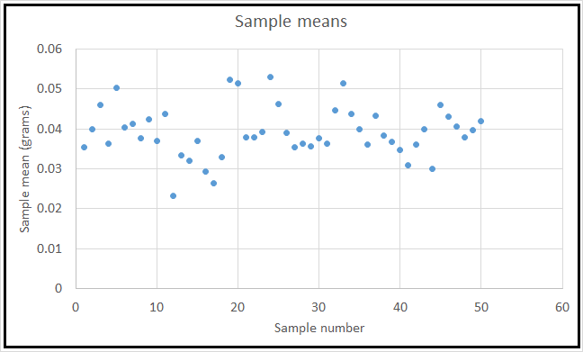
What Nature won’t readily reveal, one must infer. So I combined the contents of the two boxes, selected 30 Nerds at random (15 each of grape and strawberry), weighed this sample, computed its mean, and returned the sample to the pile.

I repeated this process 50 times and got 50 different sample means:

Some of you might recognize what I did. I was bootstrapping of course.

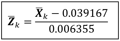
Next, I standardized each of the 50 sample means using the following formula:

Here, 0.039167 was the mean of the 50 sample means, and 0.006355 was their standard deviation.

A frequency distribution plot of the 50 standardized means revealed the following distributional shape:

The sample means appeared to be arranged neatly around the unknown (and never to be known) population mean in what looked like a normal distribution. But was the distribution really normal? How could I be sure that it wouldn’t turn into the following shape for larger sample sizes or a greater number of samples?

In the early 1800s, when Pierre-Simon Laplace was developing his ideas on what came to be known as the Central Limit Theorem, he evaluated many such distributional shapes. In fact, the one shown above was one of his favorites. Another close contender was the normal curve discovered by his fellow countryman Abraham De Moivre. You see, in those days, the normal distribution wasn’t called by its present name. And neither was its wide-ranging applicability discovered. At any rate, it definitely wasn’t regarded with the exalted level of reverence it enjoys today.

To know whether my data was indeed normally distributed, what I needed was a statistical test of normality — a test that would check whether my data obeyed the distributional properties of the normal curve. A test that would assure me that I could be X% sure that the distribution of my sample means wouldn’t crushingly morph into anything other than the normal curve were I to increase the sample size or draw a greater number of samples.

Thankfully, my need was not only a commonly felt one, but also a heavily researched one. So heavily researched is this area that during the past 100 years, scientists have invented no less than ten different tests of normality with publications still gushing out in large volume. One such test was invented in 1980 by Messieurs Carlos Jarque and Anil K. Bera. It’s based on a disarmingly simple observation. If your data were normally distributed, then its skewness (S) would be zero and kurtosis (K) would be 3 (I’ll explain what those are later in this article). Using S, K, and the sample size n, Mssrs. Jarque and Bera constructed a special random variable called JB as follows:

JB is the test statistic. The researchers proved that JB will be Chi-squared distributed with 2 degrees of freedom provided your data comes from a normally distributed population. The null hypothesis of this test is that your data is normally distributed. And the p-value of the test statistic is the probability of your data coming from a normally distributed population. Their test came to be known as the Jarque-Bera test of normality. You can also read all the JB-test in this article.

When I ran the JB-test on the set of 50 sample means, the test came back to say that I would be less than wise to reject the test’s null hypothesis. The test statistic was jb(50) = 0.30569, p = .86.

Here’s a summary of the empirical method I conducted:

1. I drew 50 random samples (with replacement) of size 30 each.
2. I calculated the sample mean X_bar_i of each sample.
3. I standardized each sample mean to get Z_bar_i.
4. I ran the JB-test of normality on the 50 standardized sample means to test if they were normally distributed.

It is common knowledge that careful scientific experimentation is an arduous and fuel-intensive endeavor, and my experiment was no exception. Hence, after my experiment was completed I helped myself to a generous serving of candy. All in the name of science obviously.

A mathematical proof of the Central Limit Theorem

There are two equally nice ways to mathematically prove the CLT, and this time I really mean prove. The first one uses the properties of Characteristic Functions. The second one uses the properties of Moment Generating Functions (MGF). The CF and the MGF are different forms of generating functions (more on that soon). The CF-based proof makes fewer assumptions than the MGF-based proof. It’s also generally speaking a solid, self-standing proof. But I won’t use it because I like MGFs more than I like CFs. So we’ll follow the line of thought adopted by Casella and Berger (see references) which uses the MGF-based approach.

Lest you are still itching to know what the CF-based proof looks like, Wikipedia has a 5-line proof of the CLT that uses Characteristic Functions, presented in the characteristically no-nonsense style of that platform. I am sure it will be a joy to go through.

Returning to the MGF-based proof, you’ll be able to appreciate it to the maximum if you know the following four concepts:

1. Sequences and series
2. The Taylor series
3. Generating Functions
4. The Moment Generating Function

I’ll begin by explaining these concepts. If you know what they are already, you can go straight to the proof, and I’ll see you there.

Sequences

A sequence is just an arrangement of stuff in some order. The figure on the left is a “bag” or a “set” (strictly speaking, a “multiset”) of Nerds. If you line up the contents of this bag, you get a sequence.

In a sequence, order matters a lot. In fact, order is everything. Remove the ordering of the elements, and they fall back to being just a bag.

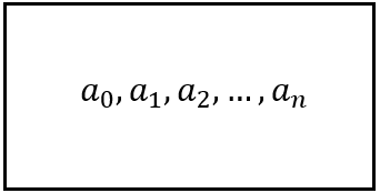
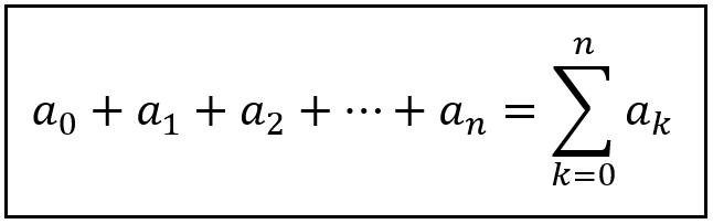
In math, a sequence of (n+1) elements is written as follows:

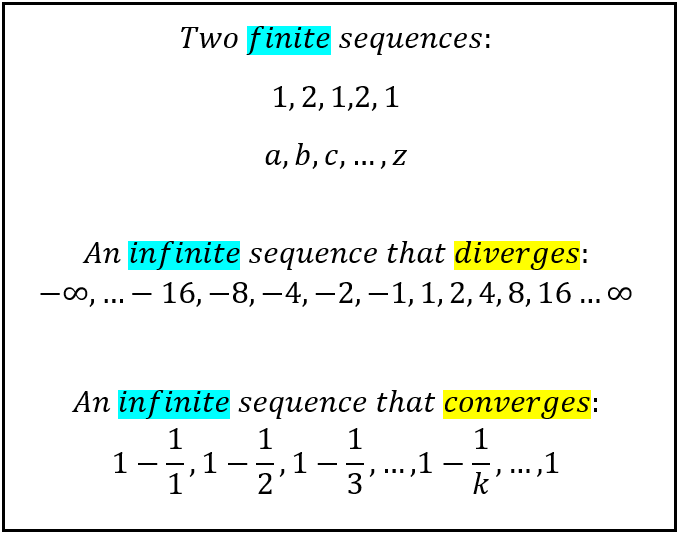
Here are some examples of sequences and their properties:

The last sequence, although containing an infinite number of terms, converges to 1, as k marches through the set of natural numbers: 1, 2, 3,…∞.

Sequences have many other fascinating properties which will be of no interest to us.

Series

Take any sequence. Now replace the comma between its elements with a plus sign. What you got yourself is a Series:

A series is finite or infinite depending on the number of terms in it. Either way, if it sums to a finite value, it’s a convergent series. Else it’s a divergent series.

Here are some examples.

In the second series, x is assumed to be finite.

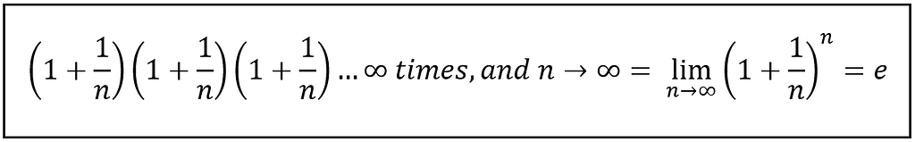
Instead of adding all elements of a sequence, if you multiply them, what you get is a product series. Perhaps the most famous example of an infinite convergent product series is the following one:

A historical footnote is in order. We assign credit for not only the above formula for ‘e’ but also to the discovery of value of ‘e’ to the 17th century Swiss mathematician Jacob Bernoulli (1655–1705), although he didn’t call it ‘e’. The name ‘e’ was reportedly given by another Swiss math genius — the great Leonhard Euler (1707–1783). If that report is true, then poor Bernoulli missed his chance to name his creation (‘b’ ?).

During the 1690s, Bernoulli also discovered the Weak Law of Large Numbers. And with that landmark discovery, he also set in motion a train of thought on limit theorems and statistical inference that kept rolling well into the 20th century. Along the way came an important discovery, namely Pierre-Simon Laplace’s discovery of the Central Limit Theorem in 1810. In what must be one of the best tributes to Jacob Bernoulli, the final step in the (modern) proof of the Central Limit Theorem, the step that links the entire chain of derivations lying before it with the final revelation of normality, relies upon the very formula for ‘e’ that Bernoulli discovered in the late 1600s.

Let’s return to our parade of topics. An infinite series forms the basis for generating functions which is the topic I will cover next.

Generating Functions

The trick to understanding Generating Function is to appreciate the usefulness of a…Label Maker.

Imagine that your job is to label all the shelves of newly constructed libraries, warehouses, storerooms, pretty much anything that requires an extensive application of labels. Anytime they build a new warehouse in Boogersville or revamp a library in Belchertown (I am not entirely making these names up), you get a call to label its shelves.

So imagine then that you just got a call to label out a shiny new warehouse. The aisles in the warehouse go from 1 through 26, and each aisle runs 50 spots deep and 5 shelves tall.

You could just print out 6500 labels like so:

A.1.1, A.1.2,…,A.1.5, A.2.1,…A.2.5,…,A50.1,…,A50.5,
B1.1,…B2.1,…,B50.5,.. and so on until Z.50.5,

And you could present yourself along with your suitcase stuffed with 6500 florescent dye coated labels at your local airport for a flight to Boogersville. It might take you a while to get through airport security.

Or here’s an idea. Why not program the sequence into your label maker? Just carry the label maker with you. At Boogersville, load the machine with a roll of tape, and off you go to the warehouse. At the warehouse, you press a button on the machine, and out flows the entire sequence for aisle ‘A’.

Your label maker is the generating function for this, and other sequences like this one:

A.1.1, A.1.2,…,A.1.5, A.2.1,…A.2.5,…,A50.1,…,A50.5

In math, a generating function is a mathematical function that you design for generating sequences of your choosing so that you don’t have to remember the entire sequence.

If your proof uses a sequence of some kind, it’s often easier to substitute the sequence with its generating function. That instantly saves you the trouble of lugging around the entire sequence across your proof. Any operations, like differentiation, that you planned to perform on the sequence, you can instead perform them on its generating function.

But wait there’s more. All of the above advantages are magnified whenever the generating sequence has a closed form like the formula for e to the power x that we saw earlier.

A really simple generating function is the one shown in the figure below for the following infinite sequence: 1,1,1,1,1,…:

As you can see, a generating sequence is actually a series.

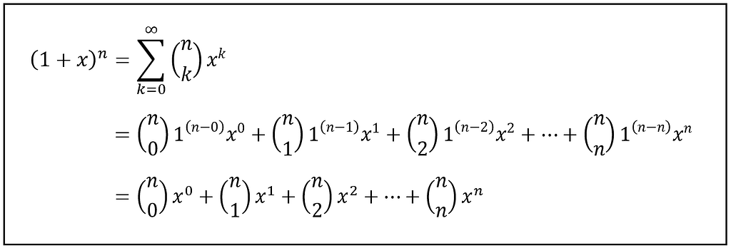
A slightly more complex generating sequence, and a famous one, is the one that generates a sequence of (n+1) binomial coefficients:

Each coefficient nCk gives you the number of different ways of choosing k out of n objects. The generating function for this sequence is the binomial expansion of (1 + x) to the power n:

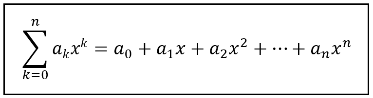
In both examples, it’s the coefficients of the x terms that constitute the sequence. The x terms raised to different powers are there primarily to keep the coefficients apart from each other. Without the x terms, the summation will just fuse all the coefficients into a single number.

The two examples of generating functions I showed you illustrate applications of the modestly named Ordinary Generating Function. The OGF has the following general form:

Another greatly useful form is the Exponential Generating Function (EGF):

It’s called exponential because the value of the factorial term in the denominator increases at an exponential rate causing the values of the successive terms to diminish at an exponential rate.

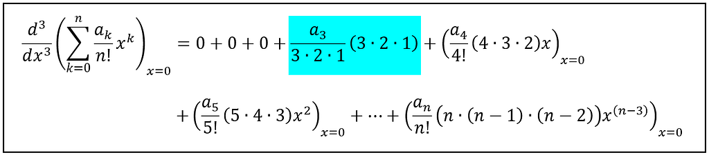
The EGF has a remarkably useful property: its k-th derivative, when evaluated at x=0 isolates out the k-th element of the sequence a_k. See below for how the 3rd derivative of the above mentioned EGF when evaluated at x=0 gives you the coefficient a_3. All other terms disappear into nothingness:

Our next topic, the Taylor series, makes use of the EGF.

Taylor series

The Taylor series is a way to approximate a function using an infinite series. The Taylor series for the function f(x) goes like this:

In evaluating the first two terms, we use the fact that 0! = 1! = 1.

f⁰(a), f¹(a), f²(a), etc. are the 0-th, 1st, 2nd, etc. derivatives of f(x) evaluated at x=a. f⁰(a) is simple f(a). The value ‘a’ can be anything as long as the function is infinitely differentiable at x = a, that is, it’s k-th derivative exists at x = a for all k from 1 through infinity.

In spite of its startling originality, the Taylor series doesn’t always work well. It creates poor quality approximations for functions such as 1/x or 1/(1-x) which march off to infinity at certain points in their domain such as at x = 0, and x = 1 respectively. These are functions with singularities in them. The Taylor series also has a hard time keeping up with functions that fluctuate rapidly. And then there are functions whose Taylor series based expansions will converge at a pace that will make continental drifts seem recklessly fast.

But let’s not be too withering of the Taylor series’ imperfections. What is really astonishing about it is that such an approximation works at all!

The Taylor series happens be to one of the most studied, and most used mathematical artifacts.

On some occasions, the upcoming proof of the CLT being one such occasion, you’ll find it useful to split the Taylor series in two parts as follows:

Here, I’ve split the series around the index ‘r’. Let’s call the two pieces T_r(x) and R_r(x). We can express f(x) in terms of the two pieces as follows:

T_r(x) is known as the Taylor polynomial of order ‘r ’ evaluated at x=a.

R_r(x) is the remainder or residual from approximating f(x) using the Taylor polynomial of order ‘r’ evaluated at x=a.

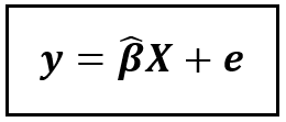
By the way, did you notice a glint of similarity between the structure of the above equation, and the general form of a linear regression model consisting of the observed value y, the modeled value β_capX, and the residual e?

But let’s not dim our focus.

Returning to the topic at hand, Taylor’s theorem, which we’ll use to prove the Central Limit Theorem, is what gives the Taylor’s series its legitimacy. Taylor’s theorem says that as x → a, the remainder term R_r(x) converges to 0 faster than the polynomial (x — a) raised to the power r. Shaped into an equation, the statement of Taylor’s theorem looks like this:

One of the great many uses of the Taylor series lies in creating a generating function for the moments of random variable. Which is what we’ll do next.

Moments and the Moment Generating Function

The k-th moment of a random variable X is the expected value of X raised to the k-th power.

This is known as the k-th raw moment.

The k-th moment of X around some value c is known as the k-th central moment of X. It’s simply the k-th raw moment of (X — c):

The k-th standardized moment of X is the k-th central moment of X divided by k-th power of the standard deviation of X:

The first 5 moments of X have specific values or meanings attached to them as follows:

• The zeroth’s raw and central moments of X are E(X⁰) and E[(X — c)⁰] respectively. Both equate to 1.
• The 1st raw moment of X is E(X). It’s the mean of X.
• The second central moment of X around its mean is E[X — E(X)]². It’s the variance of X.
• The third and fourth standardized moments of X are E[X — E(X)]³/σ³, and E[X — E(X)]⁴/σ⁴. They are the skewness and kurtosis of X respectively. Recall that skewness and kurtosis of X are used by the Jarque-Bera test of normality to test if X is normally distributed.

After the 4th moment, the interpretations become assuredly murky.

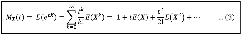
With so many moments flying around, wouldn’t it be terrific to have a generating function for them? That’s what the Moment Generating Function (MGF) is for. The Taylor series makes it super-easy to create the MGF. Let’s see how to create it.

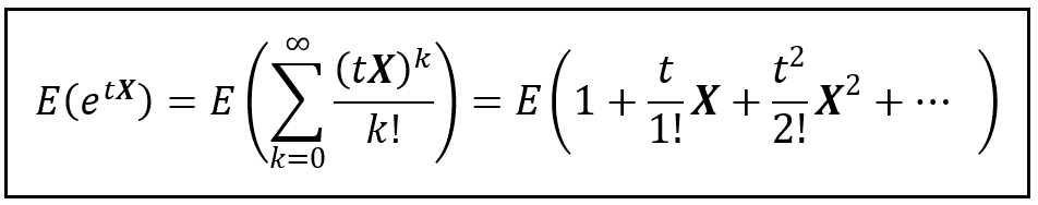
We’ll define a new random variable tX where t is a real number. Here’s the Taylor series expansion of e to the power tX evaluated at t = 0:

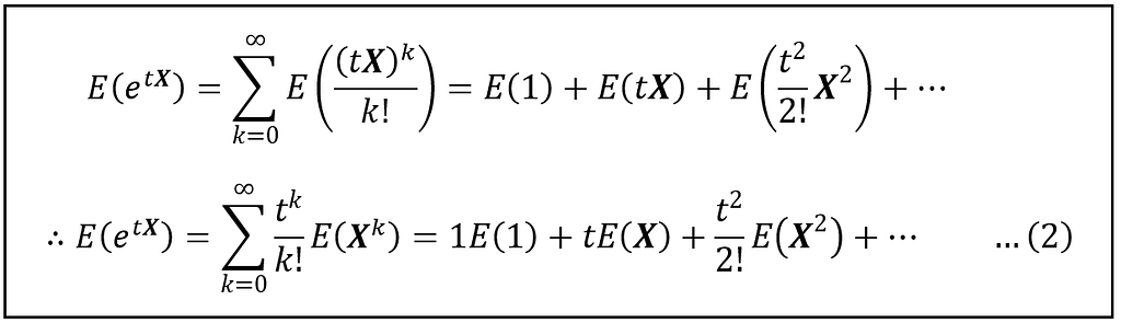
Let’s apply the Expectation operator on both sides of the above equation:

By linearity (and scaling) rule of expectation: E(aX + bY) = aE(X) + bE(Y), we can move the Expectation operator inside the summation as follows:

Recall that E(X^k] are the raw moments of X for k = 0,1,23,…

Let’s compare Eq. (2) with the general form of an Exponential Generating Function:

What do we observe? We see that E(X^k] in Eq. (2) are the coefficients a_k in the EGF. Thus Eq. (2) is the generating function for the moments of X, and so the formula for the Moment Generating Function of X is the following:

The MGF has many interesting properties. We’ll use a few of them in our proof of the Central Limit Theorem.

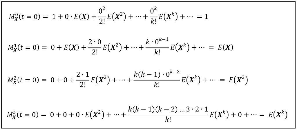
Remember how the k-th derivative of the EGF when evaluated at x = 0 gives us the k-th coefficient of the underlying sequence? We’ll use this property of the EGF to pull out the moments of X from its MGF.

The zeroth derivative of the MGF of X evaluated at t = 0 is obtained by simply substituting t = 0 in Eq. (3). M⁰_X(t=0) evaluates to 1. The first, second, third, etc. derivatives of the MGF of X evaluated at t = 0 are denoted by M¹_X(t=0), M²_X(t=0), M³_X(t=0), etc. They evaluate respectively to the first, second, third etc. raw moments of X as shown below:

This gives us our first interesting and useful property of the MGF. The k-th derivative of the MGF evaluated at t = 0 is the k-th raw moment of X.

The second property of MGFs which we’ll find useful in our upcoming proof is the following: if two random variables X and Y have identical Moment Generating Functions, then X and Y have identical Cumulative Distribution Functions:

If X and Y have identical MGFs, it implies that their mean, variance, skewness, kurtosis, and all higher order moments (whatever humanly unfathomable aspects of reality those moments might represent) are all one-is-to-one identical. If every single property exhibited by the shapes of X and Y’s CDF is correspondingly the same, you’d expect their CDFs to also be identical.

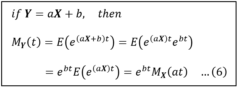
The third property of MGFs we’ll use is the following one that applies to X when X scaled by ‘a’ and translated by ‘b’:

The fourth property of MGFs that we’ll use applies to the MGF of the sum of ‘n’ independent, identically distributed random variables:

A final result, before we prove the CLT, is the MGF of a standard normal random variable N(0, 1) which is the following (you may want to compute this as an exercise):

Speaking of the standard normal random variable, as shown in Eq. (4), the first, second, third, and fourth derivatives of the MGF of N(0, 1) when evaluated at t = 0 will give you the first moment (mean) as 0, the second moment (variance) as 1, the third moment (skew) as 0, and the fourth moment (kurtosis) as 1.

And with that, the machinery we need to prove the CLT is in place.

Proof of the Central Limit Theorem

Let X_1, X_2,…,X_n be ’n’ i. i. d. random variables that form a random sample of size ’n’. Assume that we’ve drawn this sample from a population that has a mean μ and variance σ².

Let X_bar_n be the sample mean:

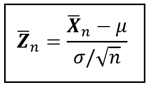
Let Z_bar_n be the standardized sample mean:

The Central Limit Theorem states that as ‘n’ tends to infinity, Z_bar_n converges in distribution to N(0, 1), i.e. the CDF of Z_bar_n becomes identical to the CDF of N(0, 1) which is often represented by the Greek letter ϕ (phi):

To prove this statement, we’ll use the property of the MGF (see Eq. 5) that if the MGFs of X and Y are identical, then so are their CDFs. Here, it’ll be sufficient to show that as n tends to infinity, the MGF of Z_bar_n converges to the MGF of N(0, 1) which as we know (see Eq. 8) is ‘e’ to the power t²/2. In short, we’d want to prove the following identity:

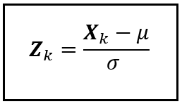
Let’s define a random variable Z_k as follows:

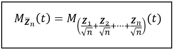
We’ll now express the standardized mean Z_bar_n in terms of Z_k as shown below:

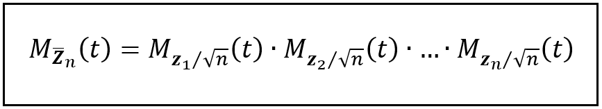
Next, we apply the MGF operator on both sides of Eq. (9):

By construction, Z_1/√n, Z_2/√n, …, Z_n/√n are independent random variables. So we can use property (7a) of MGFs which expresses the MGF of the sum of n independent random variables:

By their definition, Z_1/√n, Z_2/√n, …, Z_n/√n are also identical random variables. So we award ourselves the liberty to assume the following:

Z_1/√n = Z_2/√n = … = Z_n/√n = Z/√n.

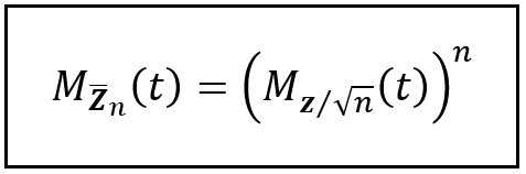
Therefore using property (7b) we get:

Finally, we’ll also use the property (6) to express the MGF of a random variable (in this case, Z) that is scaled by a constant (in this case, 1/√n) as follows:

With that, we have converted our original goal of finding the MGF of Z_bar_n into the goal of finding the MGF of Z/√n.

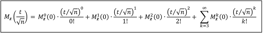
M_Z(t/√n) is a function like any other function that takes (t/√n) as a parameter. So we can create a Taylor series expansion of M_Z(t/√n) at t = 0 as follows:

Next, we split this expansion into two parts. The first part is a finite series of three terms corresponding to k = 0, k = 1, and k = 2. The second part is the remainder of the infinite series:

In the above series, M⁰, M¹, M², etc. are the 0-th, 1st, 2nd, and so on derivatives of the Moment Generating Function M_Z(t/√n) evaluated at (t/√n) = 0. We’ve seen that these derivatives of the MGF happen to be the 0-th, 1st, 2nd, etc. moments of Z.

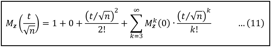
The 0-th moment, M⁰(0), is always 1. Recall that Z is, by its construction, a standard normal random variable. Hence, its first moment (mean), M¹(0), is 0, and its second moment (variance), M²(0), is 1. With these values in hand, we can express the above Taylor series expansion as follows:

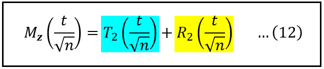
Another way to express the above expansion of M_Z is as the sum of a Taylor polynomial of order 2 which captures the first three terms of the expansion, and a residue term that captures the summation:

We’ve already evaluated the order-2 Taylor polynomial. So our task of finding the MGF of Z is now further reduced to calculating the remainder term R_2.

Before we tackle the task of computing R_2, let’s step back and review what we want to prove. We wish to prove that as the sample size ‘n’ tends to infinity, the standardized sample mean Z_bar_n converges in distribution to the standard normal random variable N(0, 1):

To prove this we realized that it was sufficient to prove that the MGF of Z_bar_n will converge to the MGF of N(0, 1) as n tends to infinity.

And that led us on a quest to find the MGF of Z_bar_n shown first in Eq. (10), and which I am reproducing below for reference:

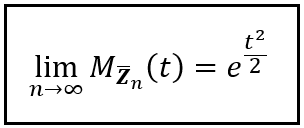
But it is really the limit of this MGF as n tends to infinity that we not only wish to calculate, but also show it to be equal to e to the power t²/2.

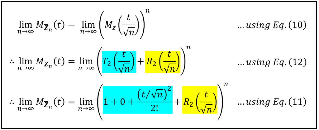
To make it to that goal, we’ll unpack and simplify the contents of Eq. (10) by sequentially applying result (12) followed by result (11) as follows:

Here we come to an uncomfortable place in our proof. Look at the equation on the last line in the above panel. You cannot just force the limit on the R.H.S. into the large bracket and zero out the yellow term. The trouble with making such a misinformed move is that there is an ‘n’ looming large in the exponent of the large bracket — the very n that wants to march away to infinity. But now get this: I said you cannot force the limit into the large bracket. I never said you cannot sneak it in.

So we shall make a sly move. We’ll show that the remainder term R_2 colored in yellow independently converges to zero as n tends to infinity no matter what its exponent is. If we succeed in that endeavor, common-sense reasoning suggests that it will be ‘legal’ to extinguish it out of the R.H.S., exponent or no exponent.

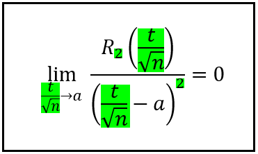
To show this, we’ll use Taylor’s theorem which I introduced in Eq. (1), and which I am reproducing below for your reference:

We’ll bring this theorem to bear upon our pursuit by setting x to (t/√n), and r to 2 as follows:

Next, we set a = 0, which instantly allows us to switch the limit:

(t/√n) → 0, to,

n → ∞, as follows:

Now we make an important and not entirely obvious observation. In the above limit, notice how the L.H.S. will tend to zero as long as n tends to infinity independent of what value t has as long as it’s finite. In other words, the L.H.S. will tend to zero for any finite value of t since the limiting behavior is driven entirely by the (√n)² in the denominator. With this revelation comes the luxury to drop t² from the denominator without changing the limiting behavior of the L.H.S. And while we’re at it, let’s also swing over the (√n)² to the numerator as follows:

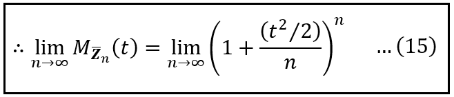
Let this result hang in your mind for a few seconds, for you’ll need it shortly. Meanwhile, let’s return to the limit of the MGF of Z_bar_n as n tends to infinity. We’ll make some more progress on simplifying the R.H.S of this limit, and then sculpting it into a certain shape:

It may not look like it, but with Eq. (14), we are literally two steps away from proving the Central Limit Theorem.

All thanks to Jacob Bernoulli’s blast-from-the-past discovery of the product-series based formula for ‘e’.

So this will be the point to fetch a few balloons, confetti, party horns or whatever.

Ready?

Here, we go:

We’ll use Eq. (13) to extinguish the green colored term in Eq. (14):

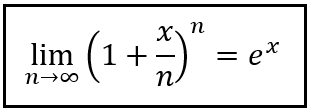
Next we’ll use the following infinite product series for (e to the power x):

Get your party horns ready.

In the above equation, set x = t²/2 and substitute this result in the R.H.S. of Eq. (15), and you have proved the Central Limit Theorem:

References and Copyrights

Books and Papers

G. Casella, R. L. Berger, “Statistical inference”, 2nd edition, Cengage Learning, 2018

Images and Videos

All images and videos in this article are copyright Sachin Date under CC-BY-NC-SA, unless a different source and copyright are mentioned underneath the image or video.

To the extent required by trademark laws, this article acknowledges Mars and NeRds to be the registered trademarks of the respective owning companies.

Thanks for reading! If you liked this article, please follow me to receive more content on statistics and statistical modeling.

---

A Proof of the Central Limit Theorem was originally published in Towards Data Science on Medium, where people are continuing the conversation by highlighting and responding to this story.

Setting A Dockerized Python Environment — The Elegant Way

This post provides a step-by-step guide for setting up a Python dockerized development environment with VScode and the Dev Containers extension.

In the previous post on this topic, Setting A Dockerized Python Environment—The Hard Way, we saw how to set up a dockerized Python development environment via the command line interface (CLI). In this post, we will review a more elegant and robust approach for setting up a dockerized Python development environment using VScode and the Dev Containers extension.

Related articles:

Setting A Dockerized Python Environment — The Hard Way

By the end of this tutorial, you will be able to set up a simple Python development environment with VScode and the Dev Containers extension.

Prerequisites

To follow along with this tutorial, you will need the following:

• Docker Desktop (or equivalent) if you are using a macOS or Windows OS machine, or Docker installed if you are using a Linux OS
• Docker Hub account to pull the image from
• VScode IDE and the Dev Containers extension installed

Throughout this tutorial, we will use the official Python image — python:3.1o.

All the code examples in this post are available here:

GitHub – RamiKrispin/vscode-python-medium: Supporting code for Medium Article

The Dev Containers Extension

Before getting started, let’s explain what the Dev Containers extension is and when you should consider using it.

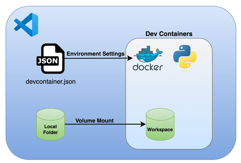
In a nutshell, the VScode Dev Containers extension enables you to open an isolated VScode session inside a docker container seamlessly. The level of isolation includes the following three layers:

• Environment
• VScode settings
• VScode extensions

The devcontainer.json file defines the session settings, enabling us to set and define the above three layers.

To set and launch your project folder inside a container with the Dev Containers extension, you will need the following two components:

• Install the Dev Containers extension
• On your project folder, create a folder named .devcontainer and set a devcontainer.json file

The below diagram describes the Dev Containers general architecture:

Upon launch, the Dev Containers extension spins a new VScode session inside a container. By default, it mounts the local folder to the container, which enables us to keep the code persistent and sync with our local folder. You can mount additional folders, but this is outside the scope of this tutorial.

In the next section, we will see how to set up a Python environment with the devcontainer.json file.

Setting a Dockerized Python Environment

Before getting started with the devcontainer.json settings, let’s first define the scope of the development environment. It should include the following features:

• Python 3.10
• Support Jupyter notebooks
• Install required libraries — Pandas and VScode Jupyter supporting libraries
• Install supporting extensions — Python and Jupyter

In the following sections, we will dive into the core functionality of the devcontainer.json file. We will start with a minimalist Python environment and demonstrate how to customize it by adding different customization layers.

Build vs. Image

The main requirement for launching a containerized session with the Dev Containers extension is to define the image settings. There are two approaches for setting the image:

• Build the image and run it during the launch time of the container with the build argument. This argument enables you to define a Dockerfile for the build and pass arguments to the docker build function. Once the build process is done, it will launch the session inside the container
• Launch the session with an existing image using the image argument

Depending on the use cases, each method has its own pros and cons. You should consider using the image argument when you have an image that fully meets the environment requirements. Likewise, a good use case for the build argument is when you have a base image but need to add minor customization settings.

In the next section, we will start with a simple example of launching a Python environment using the image argument to import the official Python image (python:3.10).

Basic Dockerized Python Environment

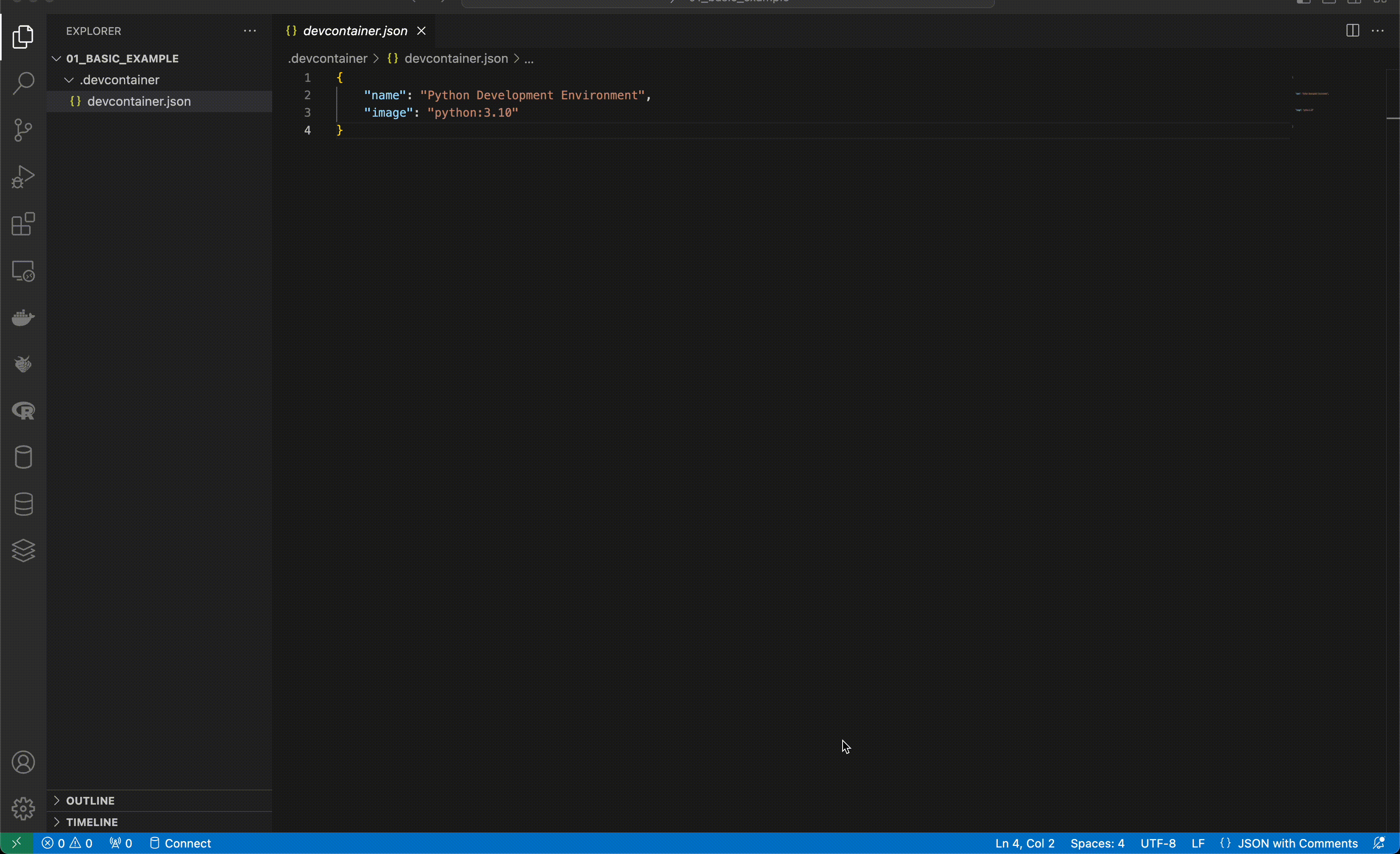
The below devcontainer.json file provides a simple example for setting up a Python environment. It uses the image argument to define the python:3.10 image as the session environment:

devcontainer.json

{
    "name": "Python Development Environment",
    "image": "python:3.10"
}

The name argument defines the environment name. In this case, we set it as Python Development Environment.

Before launching the environment, please make sure:

• Your Docker Desktop (or equivalent) is open
• You are logged in to Docker Hub (or pull in advance the Python image)
• The devcontainer.json file is set in the project folder under the .devcontainer folder:

.
└── .devcontainer
    └── devcontainer.json

The code for this example is available here.

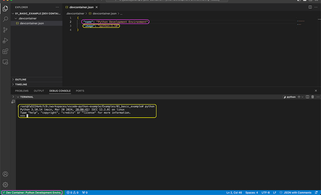
To launch a session, click the Dev Container >< symbol on the bottom left and select the Reopen in Container option as demonstrated in the screenshot below:

Note that during the first launch time of the session, the Dev Containers extension will look for the image that was defined by the image argument (in this case — python:3.10). If the image is not available locally, it will pull it from Docker Hub, and it might take a few minutes. Afterward, it should take a few seconds to launch the session.

In the above screenshot, you can see the mapping between the devcontainer.json arguments and the session settings. The session name is now available on the bottom right (marked in purple) and aligned with the value of the name argument. Likewise, the session is now running inside the python:3.10 container, and you can launch Python from the terminal.

The Python container comes with the default Python libraries. In the following section, we will see how we can add more layers on top of the Python base image with the build argument.

Customize the Python Environment with a Dockerfile

Let’s now customize the above environment by modifying the devcontainer.json. We will replace the image argument with thebuild argument. The build argument enables us to build the image during the session launch time with a Dockerfile and pass arguments to the docker build function. We will follow the same approach as demonstrated in this post to set the Python environment:

• Import the python:3.10 as the base image
• Set a virtual environment
• Install the required libraries

We will use the following Dockerfile to set the Python environment:

Dockerfile

FROM python:3.10

ARG PYTHON_ENV=my_env

ENV PYTHON_ENV=$PYTHON_ENV

RUN mkdir requirements

COPY requirements.txt set_python_env.sh /requirements/

RUN bash ./requirements/set_python_env.sh $PYTHON_ENV

We use the FROM argument to import the Python image, and the ARG and ENVarguments to set the virtual environment as an argument and environment variable. In addition, we use the following two helper files to set a virtual environment and install the required libraries:

• requirements.txt — a setting file with a list of required libraries. For this demonstration, we will install the Pandas library, version 2.0.3., and the Jupyter supporting libraries (ipykernel, ipywidgets, jupyter). The wheels library is a supporting library that handles C dependencies
• set_python_env.sh — a helper bash script that sets a virtual environment and installs the required libraries using the requirements.txt file

requirements.txt

wheel==0.40.0
pandas==2.0.3
ipykernel
ipywidgets
jupyter 

set_python_env.sh

#!/usr/bin/env bash

PYTHON_ENV=$1

python3 -m venv /opt/$PYTHON_ENV  
        && export PATH=/opt/$PYTHON_ENV/bin:$PATH 
        && echo "source /opt/$PYTHON_ENV/bin/activate" >> ~/.bashrc

source /opt/$PYTHON_ENV/bin/activate

pip3 install -r ./requirements/requirements.txt

Last but not least, we will use the following test file to evaluate if the Pandas library was installed properly and print Hello World! message:

test1.py

import pandas as pd

print("Hello World!")

Let’s make the changes in the devcontainer.json file, and replace the image argument with the build argument:

devcontainer.json

{
    "name": "Python Development Environment",
    "build": {
        "dockerfile": "Dockerfile",
        "context": ".",
        "args": {
            "PYTHON_ENV": "my_python_dev"
        }
    }
}

The files for this example are available here.

The build sub-arguments enable us to customize the image build by passing arguments to the docker build function. We use the following arguments to build the image:

• dockerfile — the path and name of the Dockerfile
• context — set the path of the local file system to enable access for files with the COPY argument during the build time. In this case, we use the current folder of the devcontainer.json file (e.g., the .devcontainer folder).
• args — set and pass arguments to the container during the build process. We use the PYTHON_ENV argument to set the virtual environment and name it as my_python_dev

You should have the three files — Dockerfile, requirements.txt, and set_python_env.sh stored under the .devcontainer folder, along with the devcontainer.json file:

.
├── .devcontainer
│   ├── Dockerfile
│   ├── devcontainer.json
│   ├── requirements.txt
│   └── set_python_env.sh
└── test2.py

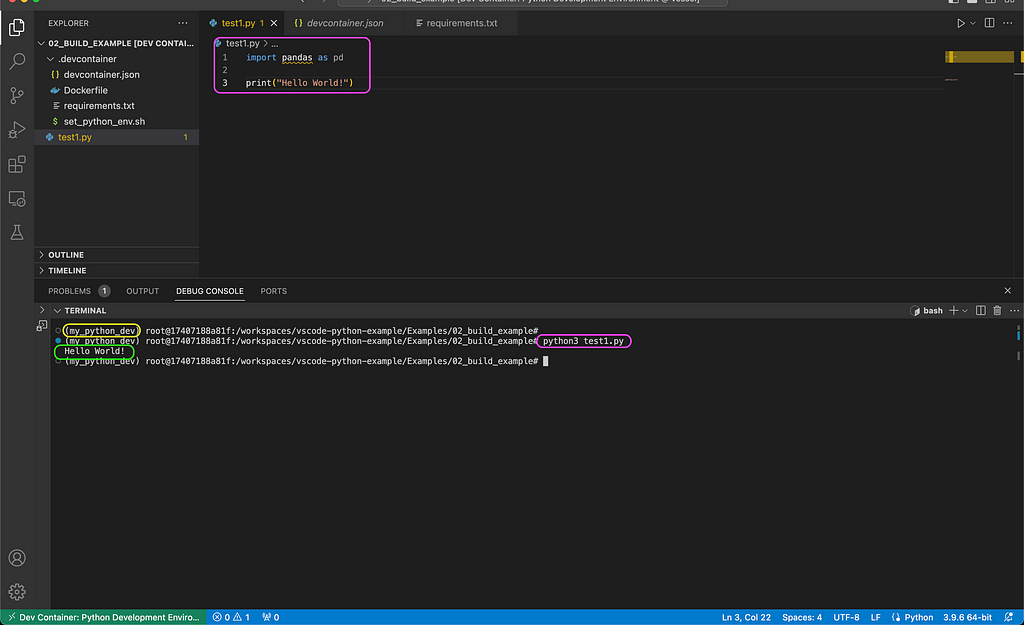
Let’s now launch the session using the new settings and test it with the test1.py file:

As you can notice in the above screenshot, we were able to successfully run the test script from the terminal (marked in purple), and it printed the Hello World! message as expected (marked in green). In addition, the virtual environment we set in the image (my_python_dev) is loaded by default (marked in yellow).

In the next section, we will see how to customize the VScode settings of the Dev Containers session.

Customize VScode Settings

One of the great features of the Dev Containers extension is that it isolates the session setting from the main VScode settings. This means you can fully customize your VScode settings at the project level. It extends the development environment’s reproducibility beyond the Python or OS settings. Last but not least, it makes collaboration with others or working on multiple machines seamless and efficient.

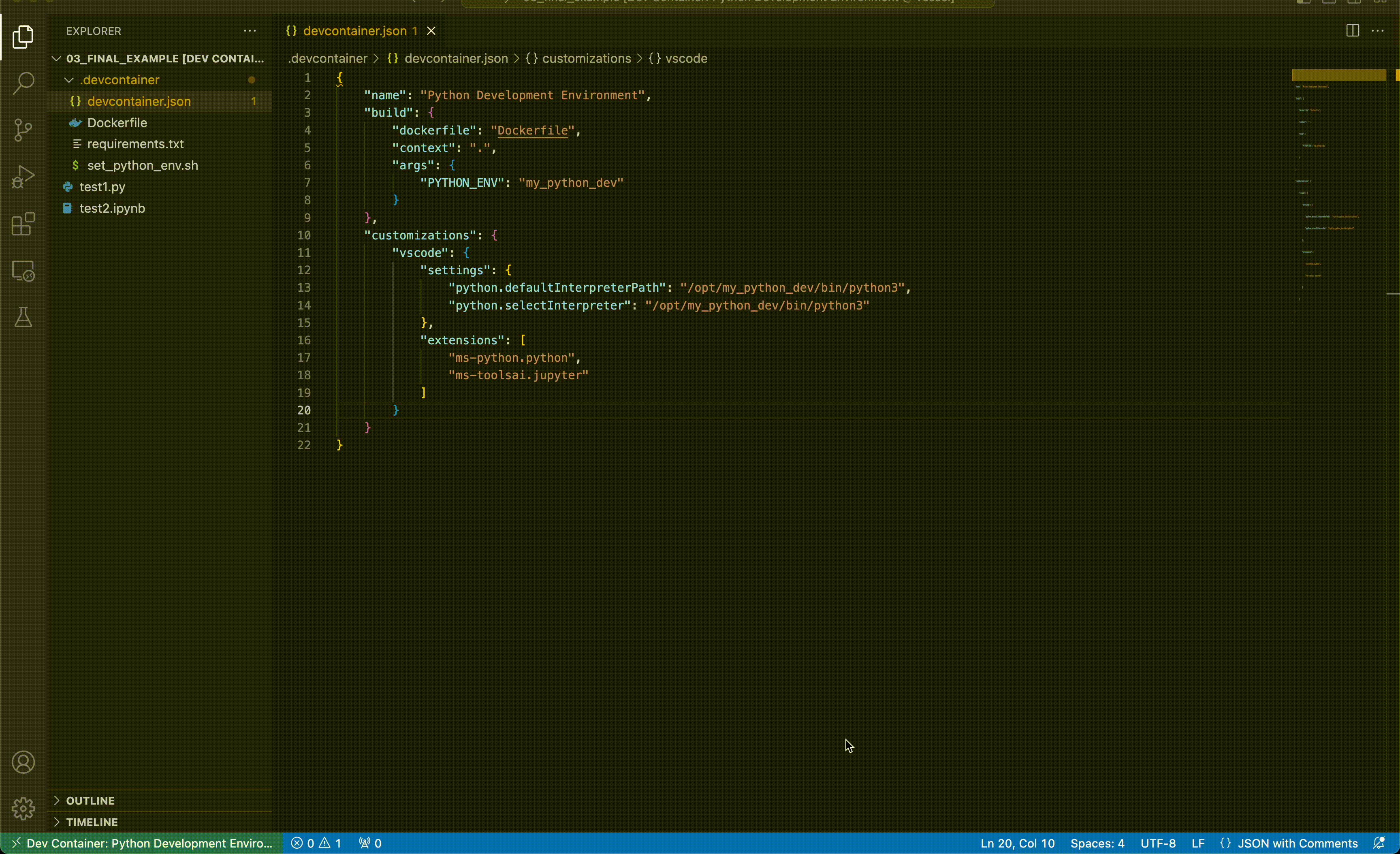
We will conclude this tutorial with the next example, where we see how to customize the VScode settings with the customizations argument. We will add the argument to the previous example and use the vscode sub-argument to set the environment default Python interpreter and the required extensions:

devcontainer.json

{
    "name": "Python Development Environment",
    "build": {
        "dockerfile": "Dockerfile",
        "context": ".",
        "args": {
            "PYTHON_ENV": "my_python_dev"
        }
    },
    "customizations": {
        "vscode": {
            "settings": {
                "python.defaultInterpreterPath": "/opt/my_python_dev/bin/python3",
                "python.selectInterpreter": "/opt/my_python_dev/bin/python3"
            },
            "extensions": [
                "ms-python.python",
                "ms-toolsai.jupyter"
            ]
        }
    }
}

The files for this example are available here.

We use the settings argument to define the Python virtual environment as defined in the image. In addition, we use the extensions argument for installing the Python and Jupyter supporting extensions.

Note: The path of the the virtual environment defined by the type of applicationas that was used to set the environment. As we use venv and named it as my_python_dev, the path is opt/my_python_dev/bin/python3.

After we add the Python extension, we can launch Python scripts using the extension plug-in, as demonstrated in the screenshot below. In addition, we can execute the Python code leveraging the Juptyer extension, in an interactive mode:

Summary

In this tutorial, we reviewed how to set a dockerized Python environment with VScode and the Dev Containers extension. The Dev Containers extension makes the integration of containers with the development workflow seamless and efficient. We saw how, with a few simple steps, we can set and customize a dockerized Python environment using the devcontainer.json file. We reviewed the two approaches for setting the session image with the image and build arguments and setting extensions with the customizations argument. There are additional customization options that were not covered in this tutorial, and I recommend checking them:

• Define environment variables
• Mount additional volumes
• Set arguments to the docker run command
• Run post-launch command

If you are interested in diving into more details, I recommend checking this tutorial:

GitHub – RamiKrispin/vscode-python: A Tutorial for Setting Python Development Environment with VScode and Docker

Resources

• Code examples — https://github.com/RamiKrispin/vscode-python-medium
• VScode — https://code.visualstudio.com/
• Dev Containers — https://code.visualstudio.com/docs/devcontainers/containers
• Setting a dockerized Python development environment with GitHub template — https://medium.com/@rami.krispin/setting-a-dockerized-python-development-environment-template-de2400c4812b

---

Setting A Dockerized Python Environment — The Elegant Way was originally published in Towards Data Science on Medium, where people are continuing the conversation by highlighting and responding to this story.