Year: 2024

An approach using Bayesian regression with brms

In neuroscience and other biomedical sciences, it is common to use behavioral tests to assess responses to experimental conditions or treatments. We can assess many aspects, from basic motor and exploratory behaviors to memory and learning. Many of these variables are continuous (numerical) responses, i.e. they can take (finite or infinite) values in a given range. Time in the open field, animal weight, or the number of cells in a brain region are some examples.

However, there are other types of variables that we record in our experiments. A very common one is ordered categorical variables, also called ordinal variables. These are categorical variables that have a natural order, analogous to the well-known surveys in which we answer whether we agree or disagree with a statement, with 0 being strongly disagree and 5 being strongly agree. To facilitate the recording of these variables in printed or digital datasheets, we codify them (by convention) as numbers. This is the case of the 5-point Bederson score used in the context of cerebral ischemia research in rodent models (1), which is coded as follows:

– 0 = no observable deficit

– 1 = forelimb flexion

– 2 = forelimb flexion and decreased resistance to lateral push

– 3 = circling

– 4 = circling and spinning around the cranial-caudal axis

– 5 = no spontaneous movement.

Note that the numbers are just simple conventions. We could also use a,b,c,d,e; excellent, good, not so good, bad, very bad, almost dead; etc. I do not think it is presumptuous to stress the self-evident nature of the matter.

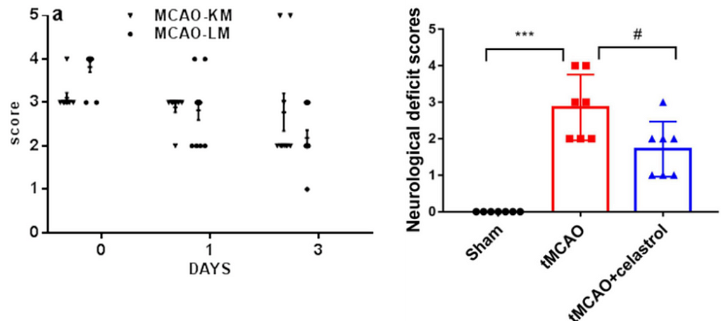
Surprisingly, however, Figure 1 represents a particular and widespread malpractice that scientists in this field have been practicing for years: They use t-tests and ANOVAS to analyze such ordered categorical variables.

I still cannot find a logical explanation for why dozens of authors, reviewers, and editors feel comfortable with this scenario. Not only is it not logical, but more importantly, it leads to biased effect sizes, low detection rates, and type I error rates, among other things (2).

When I have played the role of reviewer 2 and emphasized this point to authors, asking them why they evaluate a categorical response with a statistical test designed to deal with continuous numerical variables, what I get is a long list of published articles that follow this irrational practice. So I finally found an answer to why they do it:

what Gerd Gigerenzer (2004) calls “the ritual of mindless statistics” (3).

In fact, most of us scientists have little idea what we are doing with our data, and are simply repeating common malpractices passed down from generation to generation in labs around the world.

In this article, we’ll then look at a more viable alternative for analyzing ordered categorical variables using R, brms (4) and elements from the tidyverse (5).

Facing the ritual of mindless statistics

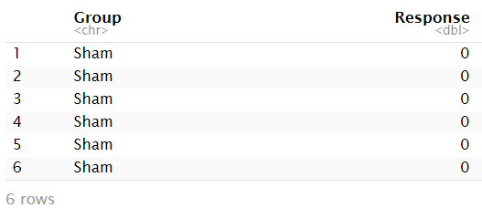
To avoid the ritual of mindless statistics, we’ll recreate the data set from Liu et. al (2022) in Figure 1 by eyeballing the data points and organizing them in a table:

# We Define the observations
observations <- list(
  Sham = c(rep(0, 7)),
  tMCAO = c(rep(2, 3), rep(3, 2), rep(4, 2)),
  tMCAO_C = c(rep(1, 3), rep(2, 3), rep(3, 1))
)

# We create an empty data frame to populate
df <- data.frame(Group = character(), Response = integer())

# We populate the data frame
for (group in names(observations)) {
  for (response in unique(observations[[group]])) {
    df <- rbind(df, data.frame(Group = rep(group, sum(observations[[group]] == response)), 
                               Response = rep(response, sum(observations[[group]] == response))))
  }
}

head(df)

If you look at the R code (in R-studio) at this point, you will notice that the variable `Response’ is identified as a number ranging from 0 to 4. Of course, we are fully aware that this response is not numeric, but an ordered (ordinal) categorical variable. So we do the conversion explicitly:

df$Response <- factor(df$Response, levels = c("0", "1", "2", "3", "4"), ordered = TRUE)

str(df)

Now we can verify that it is recognized as an ordered categorical variable. With this in hand, we can easily move on to visualization and modeling.

Exploratory data visualization

First, let’s load the necessary libraries and create a visual theme for our plots.

library(ggplot2)
library(brms)
library(ggdist)
library(easystats)
library(dplyr)
library(tibble)

Plot_theme <- theme_classic() +
  theme(
      plot.title = element_text(size=18, hjust = 0.5, face="bold"),
      plot.subtitle = element_text(size = 10, color = "black"),
      plot.caption = element_text(size = 12, color = "black"),
      axis.line = element_line(colour = "black", size = 1.5, linetype = "solid"),
      axis.ticks.length=unit(7,"pt"),
     
      axis.title.x = element_text(colour = "black", size = 16),
      axis.text.x = element_text(colour = "black", size = 16, angle = 0, hjust = 0.5),
      axis.ticks.x = element_line(colour = "black", size = 1),
      
      axis.title.y = element_text(colour = "black", size = 16),
      axis.text.y = element_text(colour = "black", size = 16),
      axis.ticks.y = element_line(colour = "black", size = 1),
      
      legend.position="right",
      legend.direction="vertical",
      legend.title = element_text(colour="black", face="bold", size=12),
      legend.text = element_text(colour="black", size=10),
      
      plot.margin = margin(t = 10,  # Top margin
                             r = 2,  # Right margin
                             b = 10,  # Bottom margin
                             l = 10) # Left margin
      ) 

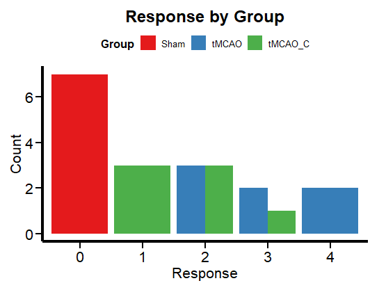
A simple way to visualize categorical data is with a bar graph.

ggplot(df, aes(x = factor(Response), fill = Group)) +
  geom_bar(position = "dodge") +
  labs(x = "Response", y = "Count", title = "Response by Group") +
  theme_minimal() +
  scale_fill_brewer(palette = "Set1") +
  Plot_theme +
theme(legend.position = "top", legend.direction = "horizontal")

Figure 2 shows the frequency per group. This is more in line with the logic of a categorical variable than box plots, which are more relevant for continuous numerical variables. Now let’s run a regression to unravel the mysteries (if any) of this data set.

Fitting an Ordinal Regression with brms

We’ll use brms to fit a cumulative model. This model assumes that the neurological score Y is derived from the categorization of a (presumably) latent (but not observable or measured) continuous variable Y˜ (2). As usual in most brms tutorials, I must apologize for skipping the “priors” issue. Let’s assume an “I have no idea” mentality and let the default (flat) brms priors do the dirty work.

We fit the cumulative model by following the usual formula syntax and adding cumulative(“probit”) as a family (assuming the latent variable and the corresponding error term are normally distributed). We have only one predictor variable, the experimental group to which each animal belongs.

Ordinal_Fit <- brm(Response ~ Group, 
           data = df, 
           family = cumulative("probit"),
           # seed for reproducibility purposes
           seed = 8807,
           control = list(adapt_delta = 0.99),
           # this is to save the model in my laptop
           file    = "Models/2024-04-03_UseAndAbuseANOVA/Ordinal_Fit.rds",
           file_refit = "never")

# Add loo for model comparison
Ordinal_Fit <- 
  add_criterion(Ordinal_Fit, c("loo", "waic", "bayes_R2"))

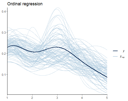
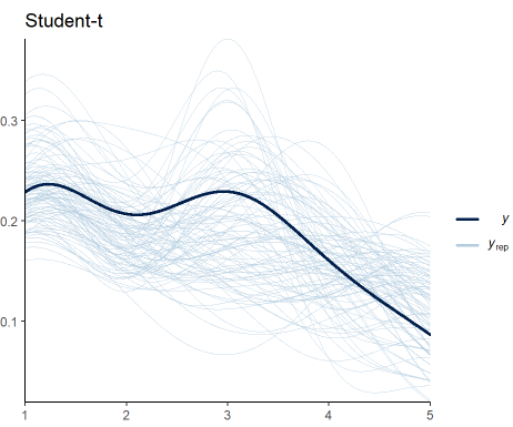
Before we look at the results, let’s do some model diagnostics to compare the observations and the model predictions.

Model diagnostics

pp_check(Ordinal_Fit, ndraws = 100) +
  labs(title = "Ordinal regression") +
  theme_classic()

From Figure 3, I speculate that such deviations are the results of the uneven distribution (variance) of scores across groups. Later, we’ll see if predicting the variance yields better estimates. For now, we are good to go.

Checking the results for the ordinal regression

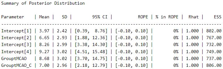
Let’s take a look at the posterior distribution using the describe_posterior function from the bayestestR package (6), as an alternative to the typical summary function.

describe_posterior(Ordinal_Fit,
                   centrality = "mean",
                   dispersion = TRUE,
                   ci_method = "HDI",
                   test = "rope",
                   )

The thresholds (score thresholds) are labeled as “Intercepts” in this model, which apply to our baseline “sham” condition. The coefficients for “GrouptMCAO” and “GrouptMCAO_C” indicate the difference from sham animals on the latent Y˜ scale. Thus, we see that “GrouptMCAO” has 8.6 standard deviations higher scores on the latent Y˜ scale.

I want to point out a crucial (and not trivial) aspect here as a reminder for a future post (stay tuned). In my opinion, it is irrelevant to make comparisons between a group that does not have a distribution (which is 0 in all cases), such as the sham group, and a group that does have a distribution (the experimental groups). If you think about it carefully, the purpose of this procedure is null. But let us follow the thread of modern scientific culture and not think too much about it.

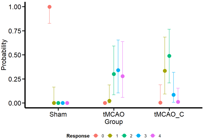
Of course, appreciating the difference between the groups becomes more feasible if we look at it visually with the conditional effects’ function ofbrms’.

Ordinal_CondEffects <- 
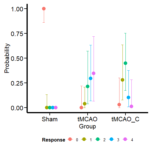
  conditional_effects(Ordinal_Fit, "Group", categorical = TRUE)

Ordinal_CondEffects <- plot(Ordinal_CondEffects, 
       plot = FALSE)[[1]]

Ordinal_CondEffects + 
  Plot_theme +
  theme(legend.position = "bottom", legend.direction = "horizontal")

Curiously (or perhaps not so much from the MCMC simulation framework), the model estimates that the dummy group can have values of 1, although we have not seen this in the data. One possible reason is that the model estimates a common variance for all groups. We’ll see if this aspect changes when we model the variance as a response.

Otherwise, the estimates obtained for the tMCAO and tMCO_C groups are much closer to the data. This allows us to make more precise statements instead of running an ANOVA (incorrectly for ordinal variables) and saying that there is “a significant difference” between one group and the other, which is a meaningless statement. For example, the model tells us that scores of 2–4 for the tMCAO group have a similar probability (about 25%). The case is different for the tMCAO_C group, where the probability of 2 in the neurological score is higher (with considerable uncertainty) than for the other scores. If I were confronted with this data set and this model, I would claim that the probability that the tMCAO_C group reflects less neurological damage (based on scores 1 and 2) is higher than for the tMCAO group.

Can we get precise numbers that quantify the differences between the scores of the different groups and their uncertainty? Of course, we can! using the emmeans package (7). But that will be the subject of another post (stay tuned).

Including the variance as a response variable

For this type of cumulative model, there is no sigma parameter. Instead, to account for unequal variances, we need to use a parameter called disc. For more on this aspect, see the Ordinal Regression tutorial by Paul-Christian Bürkner, the creator of brms (2).

Ordinal_Mdl2 <- bf (Response ~ Group) +
                     lf(disc ~  0 + Group, cmc = FALSE)

Ordinal_Fit2 <- brm( 
           formula = Ordinal_Mdl2,
           data = df, 
           family = cumulative("probit"),
           # seed for reproducibility purposes
           seed = 8807,
           control = list(adapt_delta = 0.99),
           # this is to save the model in my laptop
           file    = "Models/2024-04-03_UseAndAbuseANOVA/Ordinal_Fit2.rds",
           file_refit = "never")

# Add loo for model comparison
Ordinal_Fit2 <- 
  add_criterion(Ordinal_Fit2, c("loo", "waic", "bayes_R2"))

Model diagnostics

We perform the model diagnostics as done previously:

pp_check(Ordinal_Fit2, ndraws = 100) +
  labs(title = "Student-t") +
  theme_classic()

Figure 5 shows that my expectations were not met. Including the variance as a response in the model does not improve the fit to data. The trend is maintained, but the predictions still vary significantly. Nevertheless, this is another candidate we can consider to be our generative model.

Checking the results for our new model

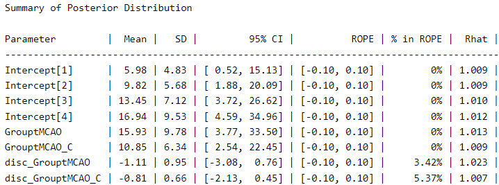
We visualize the posterior distribution for this model:

describe_posterior(Ordinal_Fit2,
                   centrality = "mean",
                   dispersion = TRUE,
                   ci_method = "HDI",
                   test = "rope",
                   )

We can see a meaningful difference in the coefficients compared to the first model. The coefficient for “GrouptMCAO” increases from 8.6 to 15.9 and that for “GrouptMCAO_C” from 7 to 10.8. Undoubtedly, this model gives us a different picture. Otherwise, the variance term is presented under the names “disc_GrouptMCAO” and “disc_GrouptMCAO_C”. We can see that both variances are very different from our “sham” baseline.

Let’s plot the results:

Ordinal_CondEffects2 <- 
  conditional_effects(Ordinal_Fit2, categorical = TRUE)

Ordinal_CondEffects2 <- plot(Ordinal_CondEffects2, 
       plot = FALSE)[[1]]

Ordinal_CondEffects2 +
  Plot_theme +
  theme(legend.position = "bottom", legend.direction = "horizontal")

Contrary to what I expected, the model still predicts that sham animals have a small probability of scoring 1. What we have confirmed here is that this prediction is not based on the (false) assumption that all groups have the same variance. Nevertheless, it is still a logical prediction (not irrational) within this framework (ordinal regression) based on thresholds. If we go to Richard McElreath’s Statistical Rethinking (8) we find the same situation with monkeys pulling levers. Fitting a more constrained model will require the use of informative priors. Leave that for a future post. I know I made three promises here, but I will keep them.

In this model, the probabilities for the different outcomes in the tMCAO group shift slightly. However, given the high uncertainty, I will not change my conclusion about the performance of this group based on this model. For the tMCAO_C group, on the other hand, the predictions do not shift in a way that is readily apparent to the eye. Let’s conclude this blog post by comparing the two models.

Model comparison

We do the model comparison using the the loo package (9, 10) for leave-one-out cross validation. For an alternative approach using the WAIC criteria (11) I suggest you read this post also published by TDS Editors.

loo(Ordinal_Fit, Ordinal_Fit2)

Under this scheme, the models have very similar performance. In fact, the first model is slightly better for out-of-sample predictions. Accounting for variance did not help much in this particular case, where (perhaps) relying on informative priors can unlock the next step of scientific inference.

I would appreciate your comments or feedback letting me know if this journey was useful to you. If you want more quality content on data science and other topics, you might consider becoming a medium member.

In the future, you may find an updated version of this post on my GitHub site.

References

1.M. Bieber, J. Gronewold, A.-C. Scharf, M. K. Schuhmann, F. Langhauser, S. Hopp, S. Mencl, E. Geuss, J. Leinweber, J. Guthmann, T. R. Doeppner, C. Kleinschnitz, G. Stoll, P. Kraft, D. M. Hermann, Validity and Reliability of Neurological Scores in Mice Exposed to Middle Cerebral Artery Occlusion. Stroke. 50, 2875–2882 (2019).

2. P.-C. Bürkner, M. Vuorre, Ordinal Regression Models in Psychology: A Tutorial. Advances in Methods and Practices in Psychological Science. 2, 77–101 (2019).

3. G. Gigerenzer, Mindless statistics. The Journal of Socio-Economics. 33, 587–606 (2004).

4. P.-C. Bürkner, Brms: An r package for bayesian multilevel models using stan. 80 (2017), doi:10.18637/jss.v080.i01.

5. H. Wickham, M. Averick, J. Bryan, W. Chang, L. D. McGowan, R. François, G. Grolemund, A. Hayes, L. Henry, J. Hester, M. Kuhn, T. L. Pedersen, E. Miller, S. M. Bache, K. Müller, J. Ooms, D. Robinson, D. P. Seidel, V. Spinu, K. Takahashi, D. Vaughan, C. Wilke, K. Woo, H. Yutani, Welcome to the tidyverse. 4, 1686 (2019).

6. D. Makowski, M. S. Ben-Shachar, D. Lüdecke, bayestestR: Describing effects and their uncertainty, existence and significance within the bayesian framework. 4, 1541 (2019).

7. R. V. Lenth, Emmeans: Estimated marginal means, aka least-squares means (2023) (available at https://CRAN.R-project.org/package=emmeans).

8. R. McElreath, Statistical rethinking (Chapman; Hall/CRC, 2020; http://dx.doi.org/10.1201/9780429029608).

9. A. Vehtari, J. Gabry, M. Magnusson, Y. Yao, P.-C. Bürkner, T. Paananen, A. Gelman, Loo: Efficient leave-one-out cross-validation and WAIC for bayesian models (2022) (available at https://mc-stan.org/loo/).

10. A. Vehtari, A. Gelman, J. Gabry, Practical Bayesian model evaluation using leave-one-out cross-validation and WAIC. Statistics and Computing. 27, 1413–1432 (2016).

11. A. Gelman, J. Hwang, A. Vehtari, Understanding predictive information criteria for Bayesian models. Statistics and Computing. 24, 997–1016 (2013).

Avoiding abuse and misuse of T-test and ANOVA: Regression for categorical responses was originally published in Towards Data Science on Medium, where people are continuing the conversation by highlighting and responding to this story.