Year: 2024

An easy and yet powerful tool for decision making

I suppose most of us have heard the statement “correlation doesn’t imply causation” multiple times. It often becomes a problem for analysts since we frequently can see only correlations but still want to make causal conclusions.

Let’s discuss a couple of examples to understand the difference better. I would like to start with a case from everyday life rather than the digital world.

In 1975, a vast population study was launched in Denmark. It’s called the Copenhagen City Heart Study (CCHS). Researchers gathered information about 20K men and women and have been monitoring these people for decades. The initial goal of this research was to find ways to prevent cardiovascular diseases and strokes. One of the conclusions from this study is that people who reported regularly playing tennis have 9.7 years higher life expectancy.

Let’s think about how we could interpret this information. Does it mean that if a person starts playing tennis weekly today, they will increase their life expectancy by ten years? Unfortunately, not exactly. Since it’s an observational study, we should be cautious about making causal inferences. There might be some other effects. For example, tennis players are likely to be wealthier, and we know that higher wealth correlates with greater longevity. Or there could be a correlation that people who regularly do sports also care more about their health and, because of it, do all checkups regularly. So, observational research might overestimate the effect of tennis on longevity since it doesn’t control other factors.

Let’s move on to the examples closer to product analytics and our day-to-day job. The number of Customer Support contacts for a client will likely be positively correlated with the probability of churn. If customers had to contact our support ten times, they would likely be annoyed and stop using our product, while customers who never had problems and are happy with the service might never reach out with any questions.

Does it mean that if we reduce the number of CS contacts, we will increase customer retention? I’m ready to bet that if we hide contact info and significantly reduce the number of CS contacts, we won’t be able to decrease churn because the actual root cause of churn is not CS contact but customers’ dissatisfaction with the product, which leads to both customers contacting us and stopping using our product.

I hope that with these examples, you can gain some intuition about the correlation vs. causation problem.

In this article, I would like to share approaches for driving causal conclusions from the data. Surprisingly, we will be able to use the most basic tool — just a linear regression.

If we use the same linear regression for causal inference, you might wonder, what is the difference between our usual approach and causal analytics? That’s a good question. Let’s start our causal journey by understanding the differences between approaches.

Predictive vs. causal analytics

Predictive analytics helps to make forecasts and answer questions like “How many customers will we have in a year if nothing changes?” or “What is the probability for this customer to make a purchase within the next seven days?”.

Causal analytics tries to understand the root causes of the process. It might help you to answer “what if” questions like “How many customers will churn if we increase our subscription fee?” or “How many customers would have signed up for our subscription if we didn’t launch this Saint Valentine’s promo?”.

Causal questions seem way more complicated than just predictive ones. However, these two approaches often leverage the same tools, such as linear or logistic regressions. Even though tools are the same, they have absolutely different goals:

• For predictive analytics, we try our best to predict a value in the future based on information we know. So, the main KPI is an error in the prediction.
• Building a regression model for the causal analysis, we focus on the relationships between our target value and other factors. The model’s main output is coefficients rather than forecasts.

Let’s look at a simple example. Suppose we would like to forecast the number of active customers.

• In the predictive approach, we are talking about baseline forecast (given that the situation will stay pretty much the same). We can use ARIMA (Autoregressive Integrated Moving Average) and base our projections on previous values. ARIMA works well for predictions but can’t tell you anything about the factors affecting your KPI and how to improve your product.
• In the case of causal analytics, our goal is to find causal relationships in our data, so we will build a regression and identify factors that can impact our KPI, such as subscription fees, marketing campaigns, seasonality, etc. In that case, we will get not only the BAU (business as usual) forecast but also be able to estimate different “what if” scenarios for the future.

Now, it’s time to dive into causal theory and learn basic terms.

Correlation doesn’t imply causation

Let’s consider the following example for our discussion. Imagine you sent a discount coupon to loyal customers of your product, and now you want to understand how it affected their value (money spent on the product) and retention.

One of the most basic causal terms is treatment. It sounds like something related to the medicine, but actually, it’s just an intervention. In our case, it’s a discount. We usually define treatment at the unit level (in our case, customer) in the following way.

The other crucial term is outcome Y, our variable of interest. In our example, it’s the customer’s value.

The fundamental problem of causal inference is that we can’t observe both outcomes for the same customers. So, if a customer received the discount, we will never know what value or retention he would have had without a coupon. It makes causal inference tricky.

That’s why we need to introduce another concept — potential outcomes. The outcome that happened is usually called factual, and the one that didn’t is counterfactual. We will use the following notation for it.

The main goal of causal analysis is to measure the relationship between treatment and outcome. We can use the following metrics to quantify it:

• ATE — average treatment effect,
• ATT — average treatment effect on treated (customers with the treatment)

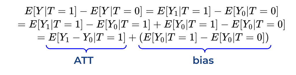
They are both equal to expected values of the differences between potential outcomes either for all units (customers in our case) or only for treated ones.

That’s an actual causal effect, and unfortunately, we won’t be able to calculate it. But cheer up; we can still get some estimations. We can observe the difference between values for treated and not treated customers (correlation effect). Let’s try to interpret this value.

Using a couple of simple mathematical transformations (i.e. adding and subtracting the same value), we’ve concluded that the average in values between treated and not treated customers equals the sum of ATT (average treatment effect on treated) and bias term. The bias equals the difference between control and treatment groups without a treatment.

If we return to our case, the bias will be equal to the difference between expected customer value for the treatment group if they haven’t received discount (counterfactual outcome) and the control group (factual outcome).

In our example, the average value from customers who received a discount will likely be much higher than for those who didn’t. Could we attribute all this effect to our treatment (discount coupon)? Unfortunately not. Since we sent discount to loyal customers who are already spending a lot of money in our product, they would likely have higher value than control group even without a treatment. So, there’s a bias, and we can’t say that the difference in value between two segments equals ATT.

Let’s think about how to overcome this obstacle. We can do an A/B test: randomly split our loyal customers into two groups and send discount coupons only to half of them. Then, we can estimate the discount’s effect as the average difference between these two groups since we’ve eliminated bias (without treatment, there’s no difference between these groups except for discount).

We’ve covered the basic theory of causal inference and have learned the most crucial concept of bias. So, we are ready to move on to practice. We will start by analysing the A/B test results.

Use case: A/B test

Randomised controlled trial (RTC), often called the A/B test, is a powerful tool for getting causal conclusions from data. This approach assumes that we are assigning treatment randomly, and it helps us eliminate bias (since groups are equal without treatment).

To practice solving such tasks, we will look at the example based on synthetic data. Suppose we’ve built an LLM-based tool that helps customer support agents answer questions more quickly. To measure the effect, we introduced this tool to half of the agents, and we would like to measure how our treatment (LLM-based tool) affects the outcome (time the agent spends answering a customer’s question).

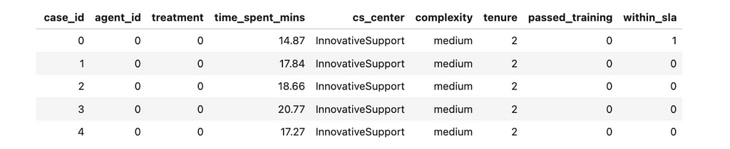
Let’s have a quick look at the data we have.

Here are the description of the parameters we logged:

• case_id — unique ID for the case.
• agent_id — unique ID for the agent.
• treatment equals 1 if agent was in an experiment group and have a chance to use LLMs, 0 — otherwise.
• time_spent_mins — minutes spent answering the customer’s question.
• cs_center — customer support centre. We are working with several CS centres. We launched this experiment in some of them because it’s easier to implement. Such an approach also helps us to avoid contamination (when agents from experiment and control groups interact and can affect each other).
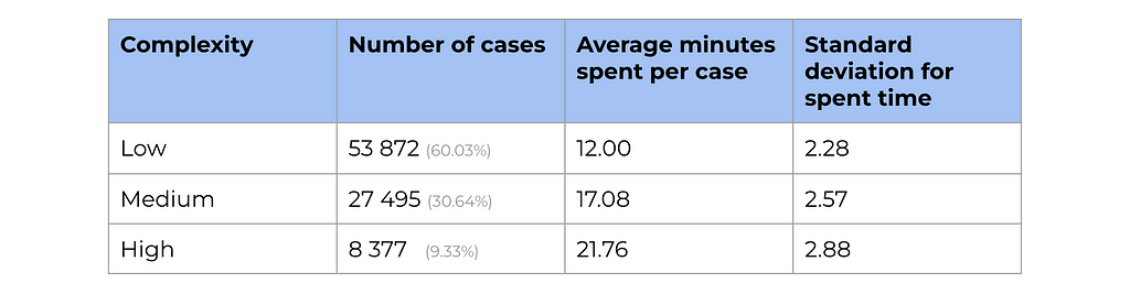
• complexity equals low, medium or high. This feature is based on the category of the customer’s question and defines how much time an agent is supposed to spend solving this case.
• tenure — number of months since the agent started working.
• passed_training — whether the agent passed LLM training. This value can be equal to True only for the treatment group since this training wasn’t offered to the agents from the control group.
• within_sla equals 1 if the agent was able to answer the question within SLA (15 minutes).

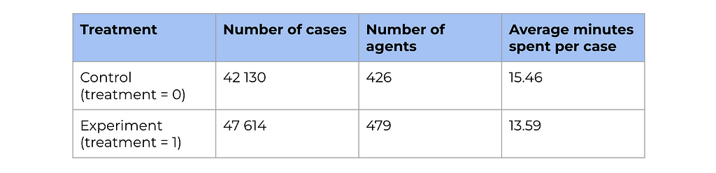
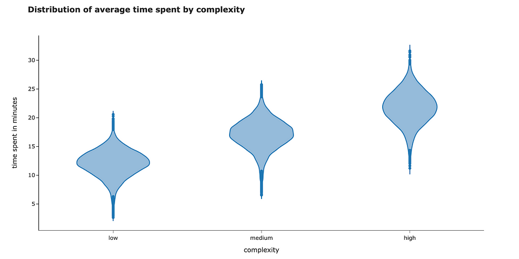
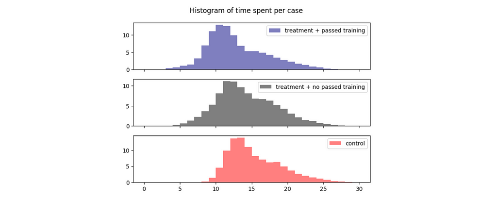
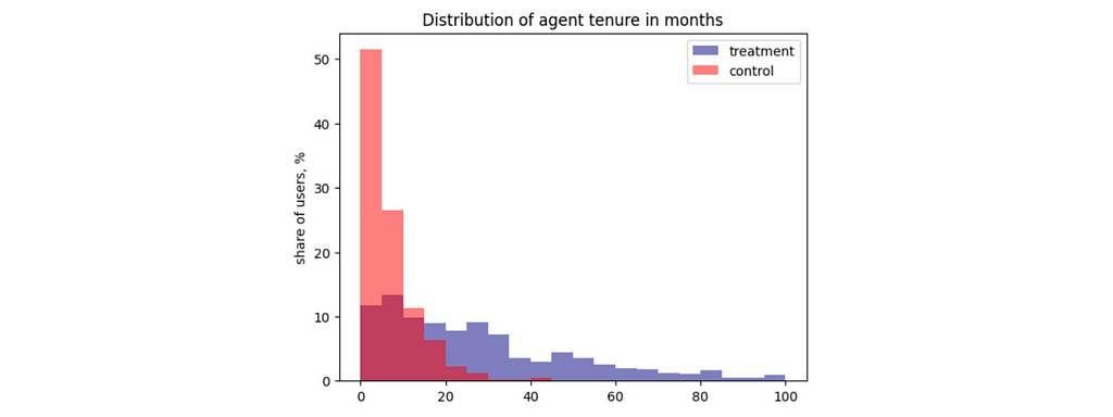
As usual, let’s start with a high-level overview of the data. We have quite a lot of data points, so we will likely be able to get statistically significant results. Also, we can see way lower average response times for the treatment group, so we can hope that the LLM tool really helps.

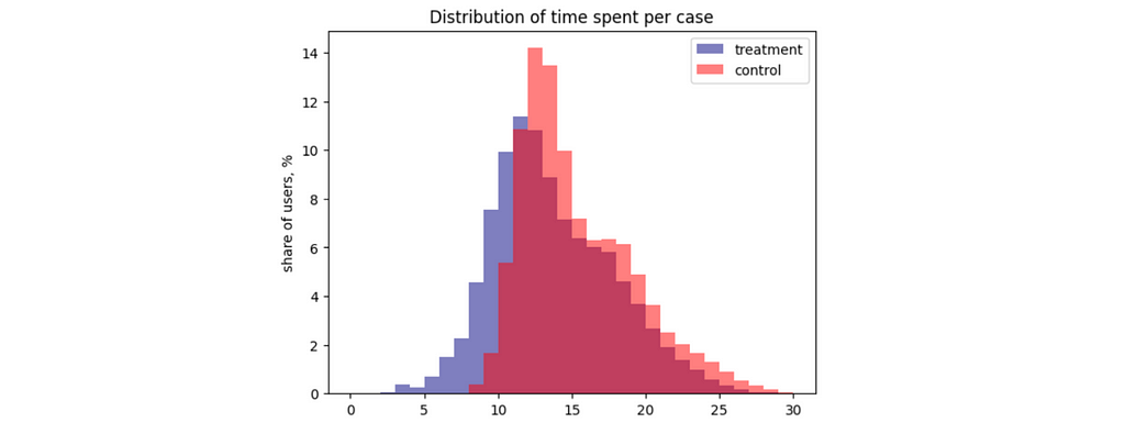
I also usually look at the actual distributions since average statistics might be misleading. In this case, we can see two unimodal distributions without distinctive outliers.

Classic statistical approach

The classic approach to analysing A/B tests is to use statistical formulas. Using the scipy package, we can calculate the confidence interval for the difference between the two means.

# defining samples
control_values = df[df.treatment == 0].time_spent_mins.values
exp_values = df[df.treatment == 1].time_spent_mins.values

# calculating p-values
from scipy.stats import ttest_ind

ttest_ind(exp_values, control_values)
# Output: TtestResult(statistic=-70.2769283935386, pvalue=0.0, df=89742.0)

We got a p-value below 1%. So, we can reject the null hypothesis and conclude that there’s a difference in average time spent per case in the control and test groups. To understand the effect size, we can also calculate the confidence interval.

from scipy import stats
import numpy as np

# Calculate sample statistics
mean1, mean2 = np.mean(exp_values), np.mean(control_values)
std1, std2 = np.std(exp_values, ddof=1), np.std(control_values, ddof=1)
n1, n2 = len(exp_values), len(control_values)
pooled_std = np.sqrt(((n1 - 1) * std1**2 + (n2 - 1) * std2**2) / (n1 + n2 - 2))
degrees_of_freedom = n1 + n2 - 2
confidence_level = 0.95

# Calculate margin of error
margin_of_error = stats.t.ppf((1 + confidence_level) / 2, degrees_of_freedom) * pooled_std * np.sqrt(1 / n1 + 1 / n2)

# Calculate confidence interval
mean_difference = mean1 - mean2
conf_interval = (mean_difference - margin_of_error, 
    mean_difference + margin_of_error)

print("Confidence Interval:", list(map(lambda x: round(x, 3), conf_interval)))
# Output: Confidence Interval: [-1.918, -1.814]

As expected since p-value is below 5%, our confidence interval doesn’t include 0.

The traditional approach works. However, we can get the same results with linear regression, which will also allow us to do more advanced analysis later. So, let’s discuss this method.

Linear regression basics

As we already discussed, observing both potential outcomes (with and without treatment) for the same object is impossible. Since we won’t be able to estimate the impact on each object individually, we need a model. Let’s assume the constant treatment effect.

Then, we can write down the relation between outcome (time spent on request) and treatment in the following way, where

• baseline is a constant that shows the basic level of outcome,
• residual represents other potential relationships we don’t care about right now (for example, the agent’s maturity or complexity of the case).

It’s a linear equation, and we can get the estimation of the impact variable using linear regression. We will use OLS (Ordinary Least Squares) function from statsmodels package.

import statsmodels.formula.api as smf
model = smf.ols('time_spent_mins ~ treatment', data=df).fit()
model.summary().tables[1]

In the result, we got all the needed info: estimation of the effect (coefficient for the treatment variable), its p-value and confidence interval.

Since the p-value is negligible (definitely below 1%), we can consider the effect significant and say that our LLM-based tool helps to reduce the time spent on a case by 1.866 minutes with a 95% confidence interval (1.814, 1.918). You can notice that we got exactly the same result as with statistical formulas before.

Adding more variables

As promised, we can make a more complex analysis with linear regression and take into account more factors, so let’s do it. In our initial approach, we used only one regressor — treatment flag. However, we can add more variables (for example, complexity).

In this case, the impact will show estimation after accounting for all the effects of other variables in the model (in our case — task complexity). Let’s estimate it. Adding more variables into the regression model is straightforward — we just need to add another component to the equation.

import statsmodels.formula.api as smf
model = smf.ols('time_spent_mins ~ treatment + complexity', data=df).fit()
model.summary().tables[1]

Now, we see a bit higher estimation of the effect — 1.91 vs 1.87 minutes. Also, the error has decreased (0.015 vs 0.027), and the confidence interval has narrowed.

You can also notice that since complexity is a categorical variable, it was automatically converted into a bunch of dummy variables. So, we got estimations of -9.8 minutes for low-complexity tasks and -4.7 minutes for medium ones.

Let’s try to understand why we got a more confident result after adding complexity. Time spent on a customer case significantly depends on the complexity of the tasks. So, complexity is responsible for a significant amount of our variable’s variability.

As I mentioned before, the coefficient for treatment estimates the impact after accounting for all the other factors in the equation. When we added complexity to our linear regression, it reduced the variance of residuals, and that’s why we got a narrower confidence interval for time.

Let’s double-check that complexity explains a significant proportion of variance. We can see a considerable decrease: time spent has a variance equal to 16.6, but when we account for complexity, it reduces to just 5.9.

time_model = smf.ols('time_spent_mins ~ complexity', data=df).fit()

print('Initial variance: %.2f' % (df.time_spent_mins.var()))
print('Residual variance after accounting for complexity: %.2f' 
  % (time_model.resid.var()))

# Output: 
# Initial variance: 16.63
# Residual variance after accounting for complexity: 5.94

So, we can see that adding a factor that can predict the outcome variable to a linear regression can improve your effect size estimations. Also, it’s worth noting that the variable is not correlated with treatment assignment (the tasks of each complexity have equal chances to be in the control or test group).

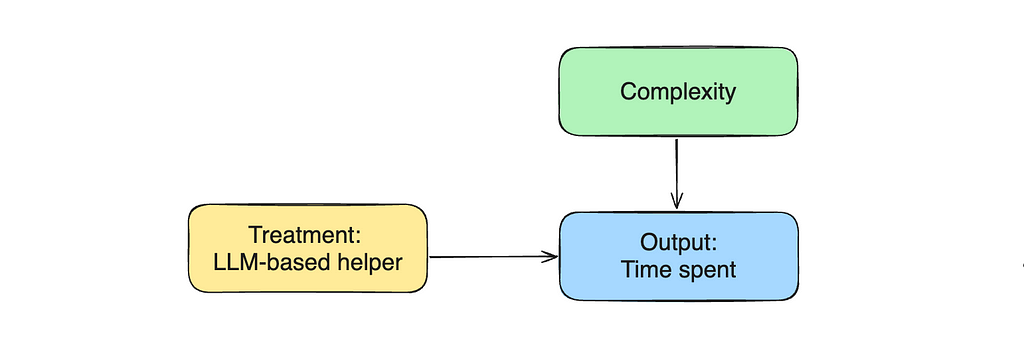
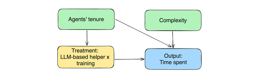
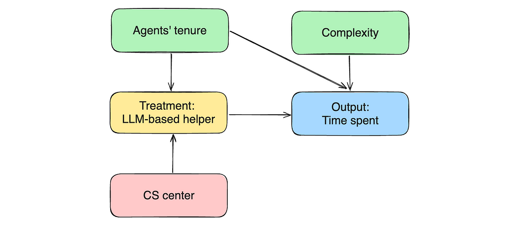
Traditionally, causal graphs are used to show the relationships between the variables. Let’s draw such a graph to represent our current situation.

Non-linear relationships

So far, we’ve looked only at linear relationships, but sometimes, it’s not enough to model our situation.

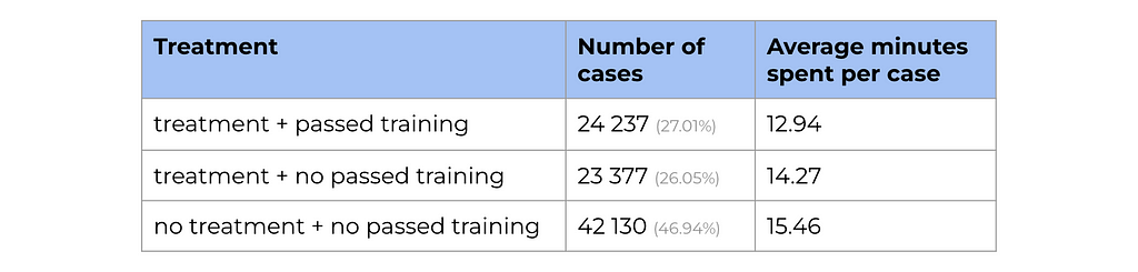
Let’s look at the data on LLM training that agents from the experiment group were supposed to pass. Only half of them have passed the LLM training and learned how to use the new tool effectively.

We can see a significant difference in average time spent for the treatment group who passed training vs. those who didn’t.

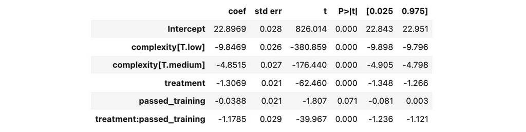
So, we should expect different impacts from treatment for these two groups. We can use non-linearity to express such relationships in formulas and add treatment * passed_training component to our equation.

model = smf.ols('time_spent_mins ~ treatment * passed_training + complexity', 
    data=df).fit()
model.summary().tables[1]

The treatment and passed_training factors will also be automatically added to the regression. So, we will be optimising the following formula.

We got the following results from the linear regression.

No statistically significant effect is associated with passed training since the p-value is above 5%, while other coefficients differ from zero.

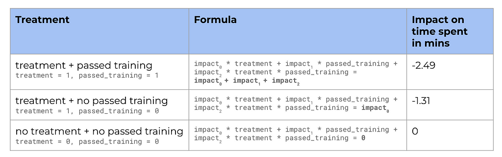
Let’s put down all the different scenarios and estimate the effects using the coefficients we got from the linear regression.

So, we’ve got new treatment estimations: 2.5 minutes improvement per case for the agents who have passed the training and 1.3 minutes — for those who didn’t.

Confounders

Before jumping to conclusions, it’s worth double-checking some assumptions we made — for example, random assignment. We’ve discussed that we launched the experiment in some CS centres. Let’s check whether agents in the different centres are similar so that our control and test groups are non-biased.

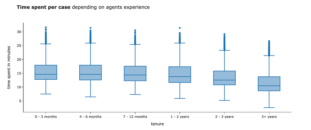
We know that agents differ by experience, which might significantly affect their performance. Our day-to-day intuition tells us that more experienced agents will spend less time on tasks. We can see in the data that it is actually like this.

Let’s see whether our experiment and control have the same level of agents’ experience. The easiest way to do it is to look at distributions.

Apparently, agents in the treatment group have much more experience than the ones in the control group. Overall, it makes sense that the product team decided to launch the experiment, starting with the more trained agents. However, it breaks our assumption about random assignment. Since the control and test groups are different even without treatment, we are overestimating the effect of our LLM tool on the agents’ performance.

Let’s return to our causal graph. The agent’s experience affects both treatment assignment and output variable (time spent). Such variables are called confounders.

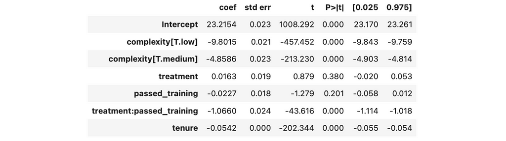
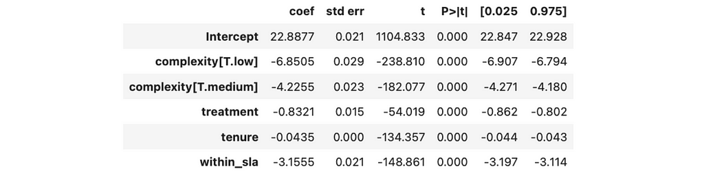
Don’t worry. We can solve this issue effortlessly — we just need to include confounders in our equation to control for it. When we add it to the linear regression, we start to estimate the treatment effect with fixed experience, eliminating the bias. Let’s try to do it.

model = smf.ols('time_spent_mins ~ treatment * passed_training + complexity + tenure', data=df).fit()
model.summary().tables[1]

With added tenure, we got the following results:

• There is no statistically significant effect of passed training or treatment alone since the p-value is above 5%. So, we can conclude that an LLM helper does not affect agents’ performance unless they have passed the training. In the previous iteration, we saw a statistically significant effect, but it was due to tenure confounding bias.
• The only statistically significant effect is for the treatment group with passed training. It equals 1.07 minutes with a 95% confidence interval (1.02, 1.11).
• Each month of tenure is associated with 0.05 minutes less time spent on the task.

We are working with synthetic data so we can easily compare our estimations with actual effects. The LLM tool reduces the time spent per task by 1 minute if the agent has passed the training, so our estimations are pretty accurate.

Bad controls

Machine learning tasks are often straightforward: you gather data with all possible features you can get, try to fit some models, compare their performance and pick the best one. Contrarily, causal inference requires some art and a deep understanding of the process you’re working with. One of the essential questions is what features are worth including in regression and which ones will spoil your results.

Till now, all the additional variables we’ve added to the linear regression have been improving the accuracy. So, you might think adding all your features to regression will be the best strategy. Unfortunately, it’s not that easy for causal inference. In this section, we will look at a couple of cases when additional variables decrease the accuracy of our estimations.

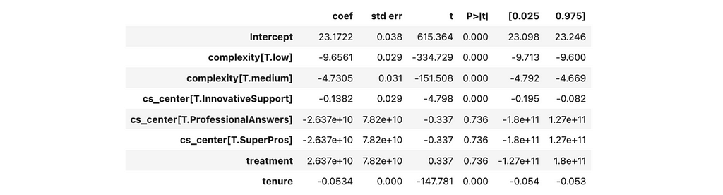
For example, we have a CS centre in data. We’ve assigned treatment based on the CS centre, so including it in the regression might sound reasonable. Let’s try.

model = smf.ols('time_spent_mins ~ treatment + complexity + tenure + cs_center', 
    data=df[df.treatment == df.passed_training]).fit()
model.summary().tables[1]

For simplicity, I’ve removed non-linearity from our dataset and equation, filtering out cases where the agents from the treatment groups didn’t pass the LLM training.

If we include the CS centre in linear regression, we will get a ridiculously high estimation of the effect (around billions) without statistical significance. So, this variable is rather harmful than helpful.

Let’s update a causal chart and try to understand why it doesn’t work. CS centre is a predictor for our treatment but has no relationship with the output variable (so it’s not a confounder). Adding a treatment predictor leads to multicollinearity (like in our case) or reduces the treatment variance (it’s challenging to estimate the effect of treatment on the output variable since treatment doesn’t change much). So, it’s a bad practice to add such variables to the equation.

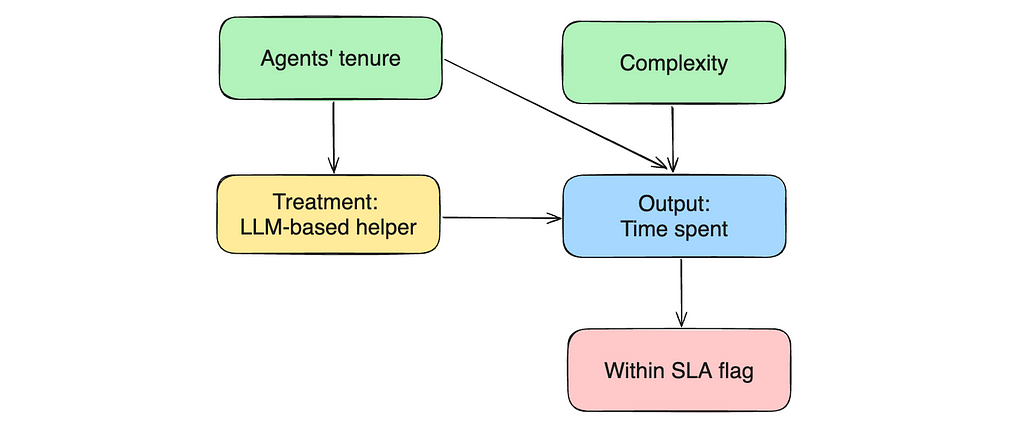
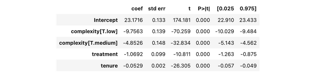
Let’s move on to another example. We have a within_sla variable showing whether the agents finished the task within 15 minutes. Can this variable improve the quality of our effect estimations? Let’s see.

model = smf.ols('time_spent_mins ~ treatment + complexity + tenure + within_sla', 
    data=df[df.treatment == df.passed_training]).fit()
model.summary().tables[1]

The new effect estimation is way lower: 0.8 vs 1.1 minutes. So, it poses a question: which one is more accurate? We’ve added more parameters to this model, so it’s more complex. Should it give more precise results, then? Unfortunately, it’s not always like that. Let’s dig deeper into it.

In this case, within_sla flag shows whether the agent solved the problem within 15 minutes or the question took more time. So, if we return to our causal chart, within_sla flag is an outcome of our output variable (time spent on the task).

When we add the within_slag flag into regression and control for it, we are starting to estimate the effect of treatment with a fixed value of within_sla. So, we will have two cases: within_sla = 1 and within_sla = 0. Let’s look at the bias for each of them.

In both cases, bias is not equal to 0, which means our estimation is biased. At first glance, it might look a bit counterintuitive. Let me explain the logic behind it a bit.

• In the first equation, we compare cases where agents finished the tasks within 15 minutes with the help of the LLM tool and without. The previous analysis shows that the LLM tool (our treatment) tends to speed up agents’ work. So, if we compare the expected time spent on tasks without treatments (when agents work independently without the LLM tool), we should expect quicker responses from the second group.
• Similarly, for the second equation, we are comparing agents who haven’t completed tasks within 15 minutes, even with the help of LLM and those who did it on their own. Again, we should expect longer response times from the first group without treatment.

It’s an example of selection bias — a case when we control for a variable on the path from treatment to output variable or outcome of the output variable. Controlling for such variables in a linear regression also leads to biased estimations, so don’t do it.

Grouped data

In some cases, you might not have granular data. In our example, we might not know the time spent on each task individually, but know the averages. It’s easier to track aggregated numbers for agents. For example, “within two hours, an agent closed 15 medium tasks”. We can aggregate our raw data to get such statistics.

agents_df = df.groupby(['agent_id', 'treatment', 'complexity', 'tenure', 
  'passed_training'], as_index = False).aggregate(
    {'case_id': 'nunique', 'time_spent_mins': 'mean'}
)

It’s not a problem for linear regression to deal with agent-level data. We just need to specify weights for each agent (equal to the number of cases).

model = smf.ols('time_spent_mins ~ treatment + complexity + tenure', 
    data = agents_df[agents_df.treatment == agents_df.passed_training],
    weights = agents_df[agents_df.treatment == agents_df.passed_training]['case_id'])
    .fit()
model.summary().tables[1]

With aggregated data, we have roughly the same results for the effect of treatment. So, there’s no problem if you have only average numbers.

Use case: observational data

We’ve looked at the A/B test examples for causal inference in detail. However, in many cases, we can’t conduct a proper randomised trial. Here are some examples:

• Some experiments are unethical. For example, you can’t push students to drink alcohol or smoke to see how it affects their performance at university.
• In some cases, you might be unable to conduct an A/B test because of legal limitations. For example, you can’t charge different prices for the same product.
• Sometimes, it’s just impossible. For example, if you are working on an extensive rebranding, you will have to launch it globally one day with a big PR announcement.

In such cases, you have to use just observations to make conclusions. Let’s see how our approach works in such a case. We will use the Student Performance data set from the UC Irvine Machine Learning Repository.

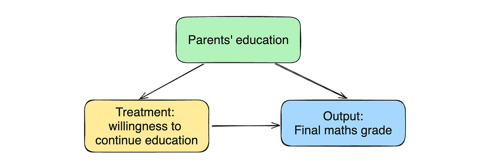
Let’s use this real-life data to investigate how willingness to take higher education affects the math class’s final score. We will start with a trivial model and a causal chart.

df = pd.read_csv('student-mat.csv', sep = ';')
model = smf.ols('G3 ~ higher', data=df).fit()
model.summary().tables[1]

We can see that willingness to continue education statistically significantly increases the final grade for the course by 3.8 points.

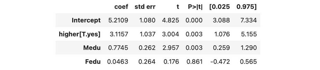
However, there might be some confounders that we have to control for. For example, parents’ education can affect both treatments (children are more likely to plan to take higher education if their parents have it) and outcomes (educated parents are more likely to help their children so that they have higher grades). Let’s add the mother and father’s education level to the model.

model = smf.ols('G3 ~ higher + Medu + Fedu', data=df).fit()
model.summary().tables[1]

We can see a statistically significant effect from the mother’s education. We likely improved the accuracy of our estimation.

However, we should treat any causal conclusions based on observational data with a pinch of salt. We can’t be sure that we’ve taken into account all confounders and that the estimation we’ve got is entirely unbiased.

Also, it might be tricky to interpret the direction of the relation. We are sure there’s a correlation between willingness to continue education and final grade. However, we can interpret it in multiple ways:

• Students who want to continue their education are more motivated, so they have higher final grades.
• Students with higher final grades are inspired by their success in studying, and that’s why they want to continue their education.

With observational data, we can only use our common sense to choose one option or the other. There’s no way to infer this conclusion from data.

Despite the limitations, we can still use this tool to try our best to come to some conclusions about the world. As I mentioned, causal inference is based significantly on domain knowledge and common sense, so it’s worth spending time near the whiteboard to think deeply about the process you’re modelling. It will help you to achieve excellent results.

You can find complete code for these examples on GitHub.

Summary

We’ve discussed quite a broad topic of causal inference, so let me recap what we’ve learned:

• The main goal of predictive analytics is to get accurate forecasts. The causal inference is focused on understanding the relationships, so we care more about the coefficients in the model than the actual predictions.
• We can leverage linear regression to get the causal conclusions.
• Understanding what features we should add to the linear regression is an art, but here is some guidance.
   — You must include confounders (features that affect both treatment and outcome).
   — Adding a feature that predicts the output variable and explains its variability can help you to get more confident estimations.
   — Avoid adding features that either affect only treatment or are the outcome of the output variable.
• You can use this approach for both A/B tests and observational data. However, with observations, we should treat our causal conclusions with a pinch of salt because we can never be sure that we accounted for all confounders.

Thank you a lot for reading this article. If you have any follow-up questions or comments, please leave them in the comments section.

Dataset

Cortez, Paulo. (2014). Student Performance. UCI Machine Learning Repository (CC BY 4.0). https://doi.org/10.24432/C5TG7T

Reference

All the images are produced by the author unless otherwise stated.

This article is inspired by the book Causal Inference for the Brave and True that gives a wonderful overview on the causal inference basics.

---

Linear Regressions for Causal Conclusions was originally published in Towards Data Science on Medium, where people are continuing the conversation by highlighting and responding to this story.

Use LangChain and OpenAI tools to extract structured information from images of receipts stored in Google Drive

This article details how we can use open source Python packages such as LangChain, pytesseract and PyPDF, along with gpt-4-vision and gpt-3.5-turbo, to identify and extract key information from images of receipts. The resulting dataset could be used for a “chat to receipts” application. Check out the full code here.

Paper receipts come in all sorts of styles and formats and represent an interesting target for automated information extraction. They also provide a wealth of itemized costs that, if aggregated into a database, could be very useful for anyone interested in tracking their spend at more detailed level than offered by bank statements.

Wouldn’t it be cool if you could take a photo of a receipt, upload it some application, then have its information extracted and appended to your personal database of expenses, which you could then query in natural language? You could then ask questions of the data like “what did I buy when I last visited IKEA?” or “what items do I spend most money on at Safeway”. Such a system might also naturally extend to corporate finance and expense tracking. In this article, we’ll build a simple application that deals with the first part of this process — namely extracting information from receipts ready to be stored in a database. Our system will monitor a Google Drive folder for new receipts, process them and append the results to a .csv file.

1. Background and motivation

Technically, we’ll be doing a type of automated information extraction called template filling. We have a pre-defined schema of fields that we want to extract from our receipts and the task will be to fill these out, or leave them blank where appropriate. One major issue here is that the information contained in images or scans of receipts is unstructured, and although Optical Character Recognition (OCR) or PDF text extraction libraries might do a decent job at finding the text, they are not good preserving the relative positions of words in a document, which can make it difficult to match an item’s price to its cost for example.

Traditionally, this issue is solved by template matching, where a pre-defined geometric template of the document is created and then extraction is only run in the areas known to contain important information. A great description of this can be found here. However, this system is inflexible. What if a new format of receipt is added?

To get around this, more advanced services like AWS Textract and AWS Rekognition use a combination of pre-trained deep learning models for object detection, bounding box generation and named entity recognition (NER). I haven’t actually tried out these services on the problem at hand, but it would be really interesting to do so in order to compare the results against what we build with OpenAI’s LLMs.

Large Language Models (LLM) such as gpt-3.5-turbo are also great at information extraction and template filling from unstructured text, especially after being given a few examples in their prompt. This makes them much more flexible than template matching or fine-tuning, since adding a few examples of a new receipt format is much faster and cheaper than re-training the model or building a new geometric template.

If we are to use gpt-3.5-turbo on text extracted from a receipts, the question then becomes how can we build the examples from which it can learn? We could of course do this manually, but that wouldn’t scale well. Here we will explore the option of using gpt-4-vision for this. This version of gpt-4 can handle conversations that include images, and appears particularly good at describing the content of images. Given an image of a receipt and a description of the key information we want to extract, gpt-4-vision should therefore be able to do the job in one shot, providing that the image is sufficiently clear.

Why wouldn’t we just use gpt-4-vision alone for this task and abandon gpt-3.5-turbo or other smaller LLMs? Technically we could, and the result might even be more accurate. But gpt-4-vision is very expensive and API calls are limited, so this system also won’t scale. Perhaps in the not-to-distant future though, vision LLMs will become a standard tool in this field of information extraction from documents.

Another motivation for this article is about exploring how we can build this system using Langchain, a popular open source LLM orchestration library. In order to force an LLM to return structured output, prompt engineering is required and Langchain has some excellent tools for this. We will also try to ensure that our system is built in a way that is extensible, because this is just the first part of what could become a larger “chat to receipts” project.

With a brief background out of the way, lets get started with the code! I will be using Python3.9 and Langchain 0.1.14 here, and full details can be found in the repo.

2. Connect to Google Drive

We need a convenient place to store our raw receipt data. Google Drive is one choice, and it provides a Python API that is relatively easy to use. To capture the receipts I use the GeniusScan app, which can upload .pdf, .jpeg or other file types from the phone directly to a Google Drive folder. The app also does some useful pre-processing such as automatic document cropping, which helps with the extraction process.

To set up API access to Google Drive, you’ll need to create service account credentials which can be generated by following the instructions here. For reference, I created a folder in my drive called “receiptchat” and set up a key pair that enables reading of data from that folder.

The following code can be used to set up a drive service object, which gives you access to various methods to query Google Drive

import os
from googleapiclient.discovery import build
from oauth2client.service_account import ServiceAccountCredentials

class GoogleDriveService:

    SCOPES = ["https://www.googleapis.com/auth/drive"]

    def __init__(self):
        # the directory where your credentials are stored
        base_path = os.path.dirname(os.path.dirname(os.path.dirname(__file__)))
        
        # The name of the file containing your credentials
        credential_path = os.path.join(base_path, "gdrive_credential.json")
        os.environ["GOOGLE_APPLICATION_CREDENTIALS"] = credential_path

    def build(self):
        
        # Get credentials into the desired format
        creds = ServiceAccountCredentials.from_json_keyfile_name(
            os.getenv("GOOGLE_APPLICATION_CREDENTIALS"), self.SCOPES
        )  
        
        # Set up the Gdrive service object
        service = build("drive", "v3", credentials=creds, cache_discovery=False)

        return service

In our simple application, we only really need to do two things: List all the files in the drive folder and download some list of them. The following class handles this:

import io
from googleapiclient.errors import HttpError
from googleapiclient.http import MediaIoBaseDownload
import googleapiclient.discovery
from typing import List


class GoogleDriveLoader:

    # These are the types of files we want to download
    VALID_EXTENSIONS = [".pdf", ".jpeg"]

    def __init__(self, service: googleapiclient.discovery.Resource):

        self.service = service

    def search_for_files(self) -> List:
        """
        See https://developers.google.com/drive/api/guides/search-files#python
        """
      
        # This query searches for objects that are not folders and 
        # contain the valid extensions
        query = "mimeType != 'application/vnd.google-apps.folder' and ("
        for i, ext in enumerate(self.VALID_EXTENSIONS):
            if i == 0:
                query += "name contains '{}' ".format(ext)
            else:
                query += "or name contains '{}' ".format(ext)
        query = query.rstrip()
        query += ")"

        # create drive api client
        files = []
        page_token = None
        try:
            while True:
                response = (
                    self.service.files()
                    .list(
                        q=query,
                        spaces="drive",
                        fields="nextPageToken, files(id, name)",
                        pageToken=page_token,
                    )
                    .execute()
                )
                for file in response.get("files"):
                    # Process change
                    print(f'Found file: {file.get("name")}, {file.get("id")}')

                    file_id = file.get("id")
                    file_name = file.get("name")

                    files.append(
                        {
                            "id": file_id,
                            "name": file_name,
                        }
                    )

                page_token = response.get("nextPageToken", None)
                if page_token is None:
                    break

        except HttpError as error:
            print(f"An error occurred: {error}")
            files = None

        return files

    def download_file(self, real_file_id: str) -> bytes:
        """
        Downloads a single file
        """

        try:
            file_id = real_file_id
            request = self.service.files().get_media(fileId=file_id)
            file = io.BytesIO()
            downloader = MediaIoBaseDownload(file, request)
            done = False
            while done is False:
                status, done = downloader.next_chunk()
                print(f"Download {int(status.progress() * 100)}.")

        except HttpError as error:
            print(f"An error occurred: {error}")
            file = None

        return file.getvalue()

Running this gives the following:

service = GoogleDriveService().build()
loader = GoogleDriveLoader(service)
all_files loader.search_for_files() #returns a list of unqiue file ids and names 
pdf_bytes = loader.download_file({some_id}) #returns bytes for that file

Great! So now we can connect to Google Drive and bring image or pdf data onto our local machine. Next, we must process it and extract text.

3. Extract raw text from .pdfs and images

Multiple well-documented open source libraries exist to extract raw text from pdfs and images. For pdfs we will use PyPDF here, although for a more comprehensive view of similar packages I recommend this article. For images in jpeg format, we will make use of pytesseract , which is a wrapper for the tesseract OCR engine. Installation instructions for that can be found here. Finally, we also want to be able to convert pdfs into jpeg format. This can be done with the pdf2image package.

Both PyPDF and pytesseract provide high level methods for extraction of text from documents. They both also have options for tuning this. pytesseract , for example, can extract both text and boundary boxes (see here), which may be of useful in future if we want to feed the LLM more information about the format of the receipt whose text its processing. pdf2image provides a method to convert pdf bytes to jpeg image, which is exactly what we want to do here. To convert jpeg bytes to an image that can be visualized, we’ll use the PIL package.

from abc import ABC, abstractmethod
from pdf2image import convert_from_bytes
import numpy as np
from PyPDF2 import PdfReader
from PIL import Image
import pytesseract
import io

DEFAULT_DPI = 50

class FileBytesToImage(ABC):

    @staticmethod
    @abstractmethod
    def convert_bytes_to_jpeg(file_bytes):
        raise NotImplementedError

    @staticmethod
    @abstractmethod
    def convert_bytes_to_text(file_bytes):
        raise NotImplementedError


class PDFBytesToImage(FileBytesToImage):

    @staticmethod
    def convert_bytes_to_jpeg(file_bytes, dpi=DEFAULT_DPI, return_array=False):
        jpeg_data = convert_from_bytes(file_bytes, fmt="jpeg", dpi=dpi)[0]
        if return_array:
            jpeg_data = np.asarray(jpeg_data)
        return jpeg_data

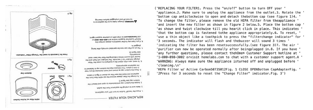
    @staticmethod
    def convert_bytes_to_text(file_bytes):
        pdf_data = PdfReader(
            stream=io.BytesIO(initial_bytes=file_bytes) 
        )
        # receipt data should only have one page
        page = pdf_data.pages[0]
        return page.extract_text()


class JpegBytesToImage(FileBytesToImage):

    @staticmethod
    def convert_bytes_to_jpeg(file_bytes, dpi=DEFAULT_DPI, return_array=False):
        jpeg_data = Image.open(io.BytesIO(file_bytes))
        if return_array:
            jpeg_data = np.array(jpeg_data)
        return jpeg_data

    @staticmethod
    def convert_bytes_to_text(file_bytes):
        jpeg_data = Image.open(io.BytesIO(file_bytes))
        text_data = pytesseract.image_to_string(image=jpeg_data, nice=1)
        return text_data

The code above uses the concept of abstract base classes to improve extensibility. Lets say we want to add support for another file type in future. If we write the associated class and inherit from FileBytesToImage , we are forced to write convert_bytes_to_image and convert_bytes_to_text methods in that. This makes it less likely that our classes will introduce errors downstream in a large application.

The code can be used as follows:

bytes_to_image = PDFBytesToImage()
image = PDFBytesToImage.convert_bytes_to_jpeg(pdf_bytes)
text = PDFBytesToImage.convert_bytes_to_jpeg(pdf_bytes)

4. Information extraction with gpt-4-vision

Now let’s use Langchain to prompt gpt-4-vision to extract some information from our receipts. We can start by using Langchain’s support for Pydantic to create a model for the output.

from langchain_core.pydantic_v1 import BaseModel, Field
from typing import List


class ReceiptItem(BaseModel):
    """Information about a single item on a reciept"""

    item_name: str = Field("The name of the purchased item")
    item_cost: str = Field("The cost of the item")


class ReceiptInformation(BaseModel):
    """Information extracted from a receipt"""

    vendor_name: str = Field(
        description="The name of the company who issued the reciept"
    )
    vendor_address: str = Field(
        description="The street address of the company who issued the reciept"
    )
    datetime: str = Field(
        description="The date and time that the receipt was printed in MM/DD/YY HH:MM format"
    )
    items_purchased: List[ReceiptItem] = Field(description="List of purchased items")
    subtotal: str = Field(description="The total cost before tax was applied")
    tax_rate: str = Field(description="The tax rate applied")
    total_after_tax: str = Field(description="The total cost after tax")

This is very powerful because Langchain can use this Pydantic model to construct format instructions for the LLM, which can be included in the prompt to force it to produce a json output with the specified fields. Adding new fields is as straightforward as just updating the model class.

Next, let’s build the prompt, which will just be static:

from dataclasses import dataclass

@dataclass
class VisionReceiptExtractionPrompt:
    template: str = """
       You are an expert at information extraction from images of receipts.

       Given this of a receipt, extract the following information:
       - The name and address of the vendor
       - The names and costs of each of the items that were purchased
       - The date and time that the receipt was issued. This must be formatted like 'MM/DD/YY HH:MM'
       - The subtotal (i.e. the total cost before tax)
       - The tax rate
       - The total cost after tax

       Do not guess. If some information is missing just return "N/A" in the relevant field.
       If you determine that the image is not of a receipt, just set all the fields in the formatting instructions to "N/A". 
       
       You must obey the output format under all circumstances. Please follow the formatting instructions exactly.
       Do not return any additional comments or explanation. 
       """

Now, we need to build a class that will take in an image and send it to the LLM along with the prompt and format instructions.

from langchain.chains import TransformChain
from langchain_core.messages import HumanMessage
from langchain_core.runnables import chain
from langchain_core.output_parsers import JsonOutputParser
import base64
from langchain.callbacks import get_openai_callback

class VisionReceiptExtractionChain:

    def __init__(self, llm):
        self.llm = llm
        self.chain = self.set_up_chain()

    @staticmethod
    def load_image(path: dict) -> dict:
        """Load image and encode it as base64."""

        def encode_image(path):
            with open(path, "rb") as image_file:
                return base64.b64encode(image_file.read()).decode("utf-8")

        image_base64 = encode_image(path["image_path"])
        return {"image": image_base64}

    def set_up_chain(self):
        extraction_model = self.llm
        prompt = VisionReceiptExtractionPrompt()
        parser = JsonOutputParser(pydantic_object=ReceiptInformation)

        load_image_chain = TransformChain(
            input_variables=["image_path"],
            output_variables=["image"],
            transform=self.load_image,
        )

        # build custom chain that includes an image
        @chain
        def receipt_model_chain(inputs: dict) -> dict:
            """Invoke model"""
            msg = extraction_model.invoke(
                [
                    HumanMessage(
                        content=[
                            {"type": "text", "text": prompt.template},
                            {"type": "text", "text": parser.get_format_instructions()},
                            {
                                "type": "image_url",
                                "image_url": {
                                    "url": f"data:image/jpeg;base64,{inputs['image']}"
                                },
                            },
                        ]
                    )
                ]
            )
            return msg.content

        return load_image_chain | receipt_model_chain | JsonOutputParser()

    def run_and_count_tokens(self, input_dict: dict):
        with get_openai_callback() as cb:
            result = self.chain.invoke(input_dict)

        return result, cb

The main method to understand here is set_up_chain , which we will walk through step by step. These steps were inspired by this blog post.

• Initialize the prompt, which in this case is just a block of text with some general instructions
• Create a JsonOutputParser from the Pydantic model we made above. This converts the model into a set of formatting instructions that can be added to the prompt
• Make a TransformChain that allows us to incorporate custom functions — in this case the load_image function — into the overall chain. Note that the chain will take in a variable called image_path and output a variable called image , which is a base64-encoded string representing the image. This is one of the formats accepted by gpt-4-vision.
• To the best of my knowledge, ChatOpenAI doesn’t yet natively support sending both text and images. Therefore, we need to make a custom chain that invokes the instance of ChatOpenAI we made with the encoded image, prompt and formatting instructions.

Note that we’re also making use of openai callbacks to count the tokens and spend associated with each call.

To run this, we can do the following:

from langchain_openai import ChatOpenAI
from tempfile import NamedTemporaryFile

model = ChatOpenAI(
  api_key={your open_ai api key},
  temperature=0, model="gpt-4-vision-preview", 
  max_tokens=1024
)

extractor = VisionReceiptExtractionChain(model)

# image from PDFBytesToImage.convert_bytes_to_jpeg()
prepared_data = {
    "image": image
}

with NamedTemporaryFile(suffix=".jpeg") as temp_file:
    prepared_data["image"].save(temp_file.name)
    res, cb = extractor.run_and_count_tokens(
        {"image_path": temp_file.name}
    )

Given our random document above, the result looks like this:

{'vendor_name': 'N/A',
 'vendor_address': 'N/A',
 'datetime': 'N/A',
 'items_purchased': [],
 'subtotal': 'N/A',
 'tax_rate': 'N/A',
 'total_after_tax': 'N/A'}

Not too exciting, but at least its structured in the correct way! When a valid receipt is provided, these fields are filled out and my assessment from running a few tests on different receipts it that its very accurate.

Our callbacks look like this:

Tokens Used: 1170
Prompt Tokens: 1104
Completion Tokens: 66
Successful Requests: 1
Total Cost (USD): $0.01302

This is essential for tracking costs, which can quickly grow during testing of a model like gpt-4.

5. Information extraction with gpt-3.5-turbo

Let’s assume that we’ve used the steps in part 4 to generate some examples and saved them as a json file. Each example consists of some extracted text and corresponding key information as defined by our ReceiptInformation Pydantic model. Now, we want to inject these examples into a call to gpt-3.5-turbo, in the hope that it can generalize what it learns from them to a new receipt. Few-shot learning is a powerful tool in prompt engineering and, if it works, would be great for this use case because whenever a new format of receipt is detected we can generate one example using gpt-4-vision and append it to the list of examples used to prompt gpt-3.5-turbo. Then when a similarly formatted receipt comes along, gpt-3.5-turbo can be used to extract its content. In a way this is like template matching, but without the need to manually define the template.

There are many ways to encourage text based LLMs to extract structured information from a block of text. One of the newest and most powerful that I’ve found is here in the Langchain documentation. The idea is to create a prompt that contains a placeholder for some examples, then inject the examples into the prompt as if they were being returned by some function that the LLM had called. This is done with the model.with_structured_output() functionality, which you can read about here. Note that this is currently in beta and so might change!

Let’s look at the code to see how this is achieved. We’ll first write the prompt.

from langchain_core.prompts import ChatPromptTemplate, MessagesPlaceholder

@dataclass
class TextReceiptExtractionPrompt:
    system: str = """
       You are an expert at information extraction from images of receipts.

       Given this of a receipt, extract the following information:
       - The name and address of the vendor
       - The names and costs of each of the items that were purchased
       - The date and time that the receipt was issued. This must be formatted like 'MM/DD/YY HH:MM'
       - The subtotal (i.e. the total cost before tax)
       - The tax rate
       - The total cost after tax

       Do not guess. If some information is missing just return "N/A" in the relevant field.
       If you determine that the image is not of a receipt, just set all the fields in the formatting instructions to "N/A". 
       
       You must obey the output format under all circumstances. Please follow the formatting instructions exactly.
       Do not return any additional comments or explanation.
       """

    prompt: ChatPromptTemplate = ChatPromptTemplate.from_messages(
        [
            (
                "system",
                system,
            ),
            MessagesPlaceholder("examples"),
            ("human", "{input}"),
        ]
    )

The prompt text is exactly the same as it was in section 4, only we now have a MessagesPlaceholder to hold the examples that we’re going to insert.

class Example(TypedDict):
    """A representation of an example consisting of text input and expected tool calls.

    For extraction, the tool calls are represented as instances of pydantic model.
    """

    input: str
    tool_calls: List[BaseModel]


class TextReceiptExtractionChain:

    def __init__(self, llm, examples: List):

        self.llm = llm
        self.raw_examples = examples
        self.prompt = TextReceiptExtractionPrompt()
        self.chain, self.examples = self.set_up_chain()

    @staticmethod
    def tool_example_to_messages(example: Example) -> List[BaseMessage]:
        """Convert an example into a list of messages that can be fed into an LLM.

        This code is an adapter that converts our example to a list of messages
        that can be fed into a chat model.

        The list of messages per example corresponds to:

        1) HumanMessage: contains the content from which content should be extracted.
        2) AIMessage: contains the extracted information from the model
        3) ToolMessage: contains confirmation to the model that the model requested a tool correctly.

        The ToolMessage is required because some of the chat models are hyper-optimized for agents
        rather than for an extraction use case.
        """
        messages: List[BaseMessage] = [HumanMessage(content=example["input"])]
        openai_tool_calls = []
        for tool_call in example["tool_calls"]:
            openai_tool_calls.append(
                {
                    "id": str(uuid.uuid4()),
                    "type": "function",
                    "function": {
                        # The name of the function right now corresponds
                        # to the name of the pydantic model
                        # This is implicit in the API right now,
                        # and will be improved over time.
                        "name": tool_call.__class__.__name__,
                        "arguments": tool_call.json(),
                    },
                }
            )
        messages.append(
            AIMessage(content="", additional_kwargs={"tool_calls": openai_tool_calls})
        )
        tool_outputs = example.get("tool_outputs") or [
            "You have correctly called this tool."
        ] * len(openai_tool_calls)
        for output, tool_call in zip(tool_outputs, openai_tool_calls):
            messages.append(ToolMessage(content=output, tool_call_id=tool_call["id"]))
        return messages

    def set_up_examples(self):

        examples = [
            (
                example["input"],
                ReceiptInformation(
                    vendor_name=example["output"]["vendor_name"],
                    vendor_address=example["output"]["vendor_address"],
                    datetime=example["output"]["datetime"],
                    items_purchased=[
                        ReceiptItem(
                            item_name=example["output"]["items_purchased"][i][
                                "item_name"
                            ],
                            item_cost=example["output"]["items_purchased"][i][
                                "item_cost"
                            ],
                        )
                        for i in range(len(example["output"]["items_purchased"]))
                    ],
                    subtotal=example["output"]["subtotal"],
                    tax_rate=example["output"]["tax_rate"],
                    total_after_tax=example["output"]["total_after_tax"],
                ),
            )
            for example in self.raw_examples
        ]

        messages = []

        for text, tool_call in examples:
            messages.extend(
                self.tool_example_to_messages(
                    {"input": text, "tool_calls": [tool_call]}
                )
            )

        return messages

    def set_up_chain(self):

        extraction_model = self.llm
        prompt = self.prompt.prompt
        examples = self.set_up_examples()
        runnable = prompt | extraction_model.with_structured_output(
            schema=ReceiptInformation,
            method="function_calling",
            include_raw=False,
        )

        return runnable, examples

    def run_and_count_tokens(self, input_dict: dict):

        # inject the examples here
        input_dict["examples"] = self.examples
        with get_openai_callback() as cb:
            result = self.chain.invoke(input_dict)

        return result, cb

TextReceiptExtractionChain is going to take in a list of examples, each of which has input and output keys (note how these are used in the set_up_examples method). For each example, we will make a ReceiptInformation object. Then we format the result into a list of messages that can be passed into the prompt. All the work in tool_examples_to_messages is there just to convert between different Langchain formats.

Running this looks very similar to what we did with the vision model:

# Load the examples 
EXAMPLES_PATH = "receiptchat/datasets/example_extractions.json"
with open(EXAMPLES_PATH) as f:
    loaded_examples = json.load(f)

loaded_examples = [
    {"input": x["file_details"]["extracted_text"], "output": x}
    for x in loaded_examples
]

# Set up the LLM caller
llm = ChatOpenAI(
  api_key=secrets["OPENAI_API_KEY"], 
  temperature=0, 
  model="gpt-3.5-turbo"
)
extractor = TextReceiptExtractionChain(llm, loaded_examples)

# convert a PDF file form Google Drive into text
text = PDFBytesToImage.convert_bytes_to_text(downloaded_data)

extracted_information, cb = extractor.run_and_count_tokens(
            {"input": text}
)

Even with 10 examples, this call is less than half the cost of the gpt-4-vision and also alot faster to return. As more examples get added, you may need to use gpt-3.5-turbo-16k to avoid exceeding the context window.

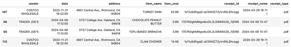
The output dataset

Having collected some receipts, you can run the extraction methods described in sections 4 and 5 and collect the result in a dataframe. This then gets stored and can be appended to whenever a new receipt appears in the Google Drive.

Once my database of extracted receipt information grows a bit larger, I plan to explore LLM-based question answering on top of it, so look out for that article soon! I’m also curious about exploring a more formal evaluation method for this project and comparing the results to what can be obtained via AWS Textract or similar products.

Thanks for making it to the end! Please feel free to explore the full codebase here https://github.com/rmartinshort/receiptchat. Any suggestions for improvement or extensions to the functionality would be much appreciated!

---

How to Build a Generative AI Tool for Information Extraction from Receipts was originally published in Towards Data Science on Medium, where people are continuing the conversation by highlighting and responding to this story.