Year: 2024

A summary of available approaches

Neural networks are indeed powerful. However, as the application scope of neural networks moves from “standard” classification and regression tasks to more complex decision-making and AI for Science, one drawback is becoming increasingly apparent: the output of neural networks is usually unconstrained, or more precisely, constrained only by simple 0–1 bounds (Sigmoid activation function), non-negative constraints (ReLU activation function), or constraints that sum to one (Softmax activation function). These “standard” activation layers have been used to handle classification and regression problems and have witnessed the vigorous development of deep learning. However, as neural networks started to be widely used for decision-making, optimization solving, and other complex scientific problems, these “standard” activation layers are clearly no longer sufficient. This article will briefly discuss the current methodologies available that can add constraints to the output of neural networks, with some personal insights included. Feel free to critique and discuss any related topics.

[中文版本(知乎)]

If one shot doesn’t work, try multiple shots

If you are familiar with reinforcement learning, you may already know what I am talking about. Applying constraints to an n-dimensional vector seems difficult, but you can break an n-dimensional vector into n outputs. Each time an output is generated, you can manually write the code to restrict the action space for the next variable to ensure its value stays within a feasible domain. This so-called “autoregressive” method has obvious advantages: it is simple and can handle a rich variety of constraints (as long as you can write the code). However, its disadvantages are also clear: an n-dimensional vector requires n calls to the network’s forward computation, which is inefficient; moreover, this method usually needs to be modeled as a Markov Decision Process (MDP) and trained through reinforcement learning, so common challenges in reinforcement learning such as large action spaces, sparse reward functions, and long training times are also unavoidable.

In the domain of solving combinatorial optimization problems with neural networks, the autoregressive method coupled with reinforcement learning was once mainstream, but it is currently being replaced by more efficient methods.

Perhaps… Let’s learn the constraints?

During training, a penalty term can be added to the objective function, representing the degree to which the current neural network output violates constraints. In the traditional optimization field, the Lagrangian dual method also offers a similar trick. Unfortunately, when applied to neural networks, these methods have so far only been proven on some simple constraints, and it is still unclear whether they are applicable to more complex constraints. One shortcoming is that inevitably some of the model’s capacity is used to learn how to meet corresponding constraints, thereby limiting the model’s ability in other directions (such as optimization solving).

For example, Karalias and Loukas, NeurIPS’21 “Erdo˝s Goes Neural: an Unsupervised Learning Framework for Combinatorial Optimization on Graphs” demonstrated that the so-called “box constraints”, where variable values lie between [a, b], can be learned through a penalty term, and the network can solve some relatively simple combinatorial optimization problems. However, our further study found that this methodology lacks generalization ability. In the training set, the neural network can maintain constraints well; but in the testing set, the constraints are almost completely lost. Moreover, although adding a penalty term in principle can apply to any constraint, it cannot handle more difficult constraints. Our paper Wang et al, ICLR’23 “Towards One-Shot Neural Combinatorial Optimization Solvers: Theoretical and Empirical Notes on the Cardinality-Constrained Case” discusses the above phenomena and presents the theoretical analysis.

On the other hand, the design philosophy of generative models, where outputs need to conform to a specific distribution, seems more suited to the “learning constraints” approach. Sun and Yang, NeurIPS’23 “DIFUSCO: Graph-based Diffusion Solvers for Combinatorial Optimization” showed that Diffusion models can output solutions that meet the constraints of the Traveling Salesman Problem (i.e., can output a complete circuit). We further presented Li et al, NeurIPS’23 “T2T: From Distribution Learning in Training to Gradient Search in Testing for Combinatorial Optimization”, where the generative model (Diffusion) is responsible for meeting constraints, with another optimizer providing optimization guidance during the gradual denoising process of Diffusion. This strategy performed pretty well in experiments, surpassing all previous neural network solvers.

Yet another interesting perspective: Solving a convex optimization problem

Maybe you are concerned that autoregressive is too inefficient, and generative models may not solve your problem. You might be thinking about a neural network that does only one forward pass, and the output needs to meet the given constraints — is that possible?

The answer is yes. We can solve a convex optimization problem to project the neural network’s output into a feasible domain bounded by convex constraints. This methodology utilizes the property that a convex optimization problem is differentiable at its KKT conditions so that this projection step can be regarded as an activation layer, embeddable in an end-to-end neural network. This methodology was proposed and promoted by Zico Kolter’s group at CMU, and they currently offer the cvxpylayers package to ease the implementation steps. The corresponding convex optimization problem is

where y is the unconstrained neural network output, x is the constrained neural network output. Because the purpose of this step is just a projection, a linear objective function can achieve this (adding an entropy regularizer is also reasonable). Ax ≤ b are the linear constraints you need to apply, which can also be quadratic or other convex constraints.

It is a personal note: there seem to be some known issues, and it seems that this repository has not been updated/maintained for a long time (04/2024). I would truly appreciate it if anyone is willing to investigate what is going on.

For non-convex problems: Which gradient approximation do you prefer?

Deriving gradients using KKT conditions is theoretically sound, but it cannot tackle non-convex or non-continuous problems. In fact, for non-continuous problems, when changes in problem parameters cause solution jumps, the real gradient becomes a delta function (i.e., infinite at the jump), which obviously can’t be used in training neural networks. Fortunately, there are some gradient approximation methods that can tackle this problem.

The Georg Martius group at Max Planck Institute introduced a black-box approximation method Vlastelica et al, ICLR’2020 “Differentiation of Blackbox Combinatorial Solvers”, which views the solver as a black box. It first calls the solver once, then perturbs the problem parameters in a specific direction, and then calls the solver again. The residual between the outputs of the two solver calls serves as the approximate gradient. If this methodology is applied to the output of neural networks to enforce constraints, we can define an optimization problem with a linear objective function:

where y is the unconstrained neural network output, and x is the constrained neural network output. Your next step is to implement an algorithm to solve the above problem (not necessarily to be optimal), and then it can be integrated into the black-box approximation framework. A drawback of the black-box approximation method is that it can only handle linear objective functions, but a linear objective function just happens to work if you are looking for some methods to enforce constraints; moreover, since it is just a gradient approximation method if the hyperparameters are not well-tuned, it might encounter sparse gradients and convergence issues.

Another method for approximating gradients involves using a large amount of random noise perturbation, repeatedly calling the solver to estimate a gradient, as discussed in Berthet et al, NeurIPS’2020 “Learning with Differentiable Perturbed Optimizers”. Theoretically, the gradient obtained this way should be similar to the gradient obtained through the LinSAT method (which will be discussed in the next section), being the gradient of an entropy-regularized linear objective function; however, in practice, this method requires a large number of random samples, which is kind of impractical (at least on my use cases).

Self-promotion time: Projection without solving optimization

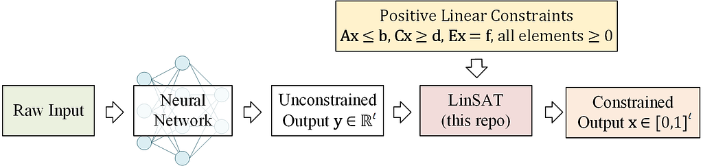
Whether it’s deriving gradients from KKT conditions for convex problems or approximating gradients for non-convex methods, both require calling/writing a solver, whereby the CPU-GPU communication could be a bottleneck because most solvers are usually designed and implemented for CPUs. Is there a way to project specific constraints directly on the GPU like an activation layer, without solving optimization problems explicitly?

The answer is yes, and our Wang et al, ICML’2023 “LinSATNet: The Positive Linear Satisfiability Neural Networks” presents a viable path and derives the convergence property of the algorithm. LinSAT stands for Linear SATisfiability Network.

LinSAT can be seen as an activation layer, allowing you to apply general positive linear constraints to the output of a neural network.

The LinSAT layer is fully differentiable, and the real gradients are computed by autograd, just like other activation layers. Our implementation now supports PyTorch.

You can install it by

pip install linsatnet

And get started with

from LinSATNet import linsat_layer

A quick example

If you download and run the source code, you will find a simple example. In this example, we apply doubly stochastic constraints to a 3×3 matrix.

To run the example, first clone the repo:

git clone https://github.com/Thinklab-SJTU/LinSATNet.git

Go into the repo, and run the example code:

cd LinSATNet
python LinSATNet/linsat.py

In this example, we try to enforce doubly-stochastic constraints to a 3×3 matrix. The doubly stochastic constraint means that all rows and columns of the matrix should sum to 1.

The 3×3 matrix is flattened into a vector, and the following positive linear constraints are considered (for Ex=f):

E = torch.tensor(
    [[1, 1, 1, 0, 0, 0, 0, 0, 0],
     [0, 0, 0, 1, 1, 1, 0, 0, 0],
     [0, 0, 0, 0, 0, 0, 1, 1, 1],
     [1, 0, 0, 1, 0, 0, 1, 0, 0],
     [0, 1, 0, 0, 1, 0, 0, 1, 0],
     [0, 0, 1, 0, 0, 1, 0, 0, 1]], dtype=torch.float32
)
f = torch.tensor([1, 1, 1, 1, 1, 1], dtype=torch.float32)

We randomly init w and regard it as the output of some neural networks:

w = torch.rand(9) # w could be the output of neural network
w = w.requires_grad_(True)

We also have a “ground-truth target” for the output of linsat_layer, which is a diagonal matrix in this example:

x_gt = torch.tensor(
    [1, 0, 0,
     0, 1, 0,
     0, 0, 1], dtype=torch.float32
)

The forward/backward passes of LinSAT follow the standard PyTorch style and are readily integrated into existing deep learning pipelines.

The forward pass:

linsat_outp = linsat_layer(w, E=E, f=f, tau=0.1, max_iter=10, dummy_val=0)

The backward pass:

loss = ((linsat_outp — x_gt) ** 2).sum()
loss.backward()

You can also set E as a sparse matrix to improve the time & memory efficiency (especially for large-sized input). Here is a dumb example (consider to construct E in sparse for the best efficiency):

linsat_outp = linsat_layer(w, E=E.to_sparse(), f=f, tau=0.1, max_iter=10, dummy_val=0)

We can also do gradient-based optimization over w to make the output of linsat_layer closer to x_gt. This is what happens when you train a
neural network.

niters = 10
opt = torch.optim.SGD([w], lr=0.1, momentum=0.9)
for i in range(niters):
 x = linsat_layer(w, E=E, f=f, tau=0.1, max_iter=10, dummy_val=0)
 cv = torch.matmul(E, x.t()).t() — f.unsqueeze(0)
 loss = ((x — x_gt) ** 2).sum()
 loss.backward()
 opt.step()
 opt.zero_grad()
 print(f’{i}/{niters}n’
 f’ underlying obj={torch.sum(w * x)},n’
 f’ loss={loss},n’
 f’ sum(constraint violation)={torch.sum(cv[cv > 0])},n’
 f’ x={x},n’
 f’ constraint violation={cv}’)

And you are likely to see the loss decreasing during the training steps.

For full API references, please check out the GitHub repository.

How does LinSAT work?

Warning, tons of math ahead! You can safely skip this part if you are just using LinSAT.

If you want to learn more details and proofs, please refer to the main paper.

Here we introduce the mechanism inside LinSAT. It works by extending the Sinkhorn algorithm to multiple sets of marginals (to our best knowledge, we are the first to study Sinkhorn with multi-sets of marginals). The positive linear constraints are then enforced by transforming the constraints into marginals.

Classic Sinkhorn with single-set marginals

Let’s start with the classic Sinkhorn algorithm. Given non-negative score matrix S with size m×n, and a set of marginal distributions on rows (non-negative vector v with size m) and columns (non-negative vector u with size n), where

the Sinkhorn algorithm outputs a normalized matrix Γ with size m×n and values in [0,1] so that

Conceptually, Γᵢ ⱼ means the proportion of uⱼ moved to vᵢ.

The algorithm steps are:

Note that the above formulation is modified from the conventional Sinkhorn formulation. Γᵢ ⱼ uⱼ is equivalent to the elements in the “transport” matrix in papers such as (Cuturi 2013). We prefer this new formulation as it generalizes smoothly to Sinkhorn with multi-set marginals in the following.

To make a clearer comparison, the transportation matrix in (Cuturi 2013) is P with size m×n, and the constraints are

Pᵢ ⱼ means the exact mass moved from uⱼ to vᵢ.

The algorithm steps are:

Extended Sinkhorn with multi-set marginals

We discover that the Sinkhorn algorithm can generalize to multiple sets of marginals. Recall that Γᵢ ⱼ ∈ [0,1] means the proportion of uⱼ moved to vᵢ. Interestingly, it yields the same formulation if we simply replace u, v with another set of marginal distributions, suggesting the potential of extending the Sinkhorn algorithm to multiple sets of marginal distributions. Denote that there are k sets of marginal distributions that are jointly enforced to fit more complicated real-world scenarios. The sets of marginal distributions are

and we have:

It assumes the existence of a normalized Z ∈ [0,1] with size m×n, s.t.

i.e., the multiple sets of marginal distributions have a non-empty feasible region (you may understand the meaning of “non-empty feasible region” after reading the next section about how to handle positive linear constraints). Multiple sets of marginal distributions could be jointly enforced by traversing the Sinkhorn iterations over k sets of marginal distributions. The algorithm steps are:

In our paper, we prove that the Sinkhorn algorithm for multi-set marginals shares the same convergence pattern with the classic Sinkhorn, and its underlying formulation is also similar to the classic Sinkhorn.

Transforming positive linear constraints into marginals

Then we show how to transform the positive linear constraints into marginals, which are handled by our proposed multi-set Sinkhorn.

Encoding neural network’s output
For an l-length vector denoted as y (which can be the output of a neural network, also it is the input to linsat_layer), the following matrix is built

where W is of size 2 × (l + 1), and β is the dummy variable, the default is β = 0. y is put at the upper-left region of W. The entropic regularizer is then enforced to control discreteness and handle potential negative inputs:

The score matrix S is taken as the input of Sinkhorn for multi-set marginals.

From linear constraints to marginals

1) Packing constraint Ax ≤ b. Assuming that there is only one constraint, we rewrite the constraint as

Following the “transportation” view of Sinkhorn, the output x moves at most b unit of mass from a₁, a₂, …, aₗ, and the dummy dimension allows the inequality by moving mass from the dummy dimension. It is also ensured that the sum of uₚ equals the sum of vₚ. The marginal distributions are defined as

2 ) Covering constraint Cx ≥ d. Assuming that there is only one constraint, we rewrite the constraint as

We introduce the multiplier

because we always have

(else the constraint is infeasible), and we cannot reach a feasible solution where all elements in x are 1s without this multiplier. Our formulation ensures that at least d unit of mass is moved from c₁, c₂, …, cₗ by x, thus representing the covering constraint of “greater than”. It is also ensured that the sum of u_c equals the sum of v_c. The marginal distributions are defined as

3) Equality constraint Ex = f. Representing the equality constraint is more straightforward. Assuming that there is only one constraint, we rewrite the constraint as

The output x moves e₁, e₂, …, eₗ to f, and we need no dummy element in uₑ because it is an equality constraint. It is also ensured that the sum of uₑ equals the sum of vₑ. The marginal distributions are defined as

After encoding all constraints and stacking them as multiple sets of marginals, we can call the Sinkhorn algorithm for multi-set marginals to encode the constraints.

Experimental Validation of LinSAT

In our ICML paper, we validated the LinSATNet method for routing constraints beyond the general case (used for solving variants of the Traveling Salesman Problem), partial graph matching constraints (used in graph matching where only subsets of graphs match each other), and general linear constraints (used in specific preference with portfolio optimization). All these problems can be represented with positive linear constraints and handled using the LinSATNet method. In experiments, neural networks are capable of learning how to solve all three problems.

It should be noted that the LinSATNet method can only handle positive linear constraints, meaning that it is unable to handle constraints like x₁ — x₂ ≤ 0 which contain negative terms. However, positive linear constraints already cover a vast array of scenarios. For each specific problem, the mathematical modeling is often not unique, and in many cases, a reasonable positive linear formulation could be found. In addition to the examples mentioned above, let the network output organic molecules (represented as graphs, ignoring hydrogen atoms, considering only the skeleton) can consider constraints such as C atoms having no more than 4 bonds, O atoms having no more than 2 bonds.

Afterword

Adding constraints to neural networks has a wide range of application scenarios, and so far, several methods are available. It’s important to note that there is no golden standard to judge their superiority over each other — the best method is usually relevant to a certain scenario.

Of course, I recommend trying out LinSATNet! Anyway, it is as simple as an activation layer in your network.

If you found this article helpful, please feel free to cite:

@inproceedings{WangICML23,
  title={LinSATNet: The Positive Linear Satisfiability Neural Networks},
  author={Wang, Runzhong and Zhang, Yunhao and Guo, Ziao and Chen, Tianyi and Yang, Xiaokang and Yan, Junchi},
  booktitle={International Conference on Machine Learning (ICML)},
  year={2023}
}

All aforementioned content has been discussed in this paper.

How to Encode Constraints to the Output of Neural Networks was originally published in Towards Data Science on Medium, where people are continuing the conversation by highlighting and responding to this story.