Year: 2024

Examining Longterm Machine Learning through ELLA and Voyager: Part 2 of Why LLML is the Next Game-changer of AI

Understanding the power of Lifelong Learning through the Efficient Lifelong Learning Algorithm (ELLA) and VOYAGER

I encourage you to read Part 1: The Origins of LLML if you haven’t already, where we saw the use of LLML in reinforcement learning. Now that we’ve covered where LLML came from, we can apply it to other areas, specifically supervised multi-task learning, to see some of LLML’s true power.

Supervised LLML: The Efficient Lifelong Learning Algorithm

The Efficient Lifelong Learning Algorithm aims to train a model that will excel at multiple tasks at once. ELLA operates in the multi-task supervised learning setting, with multiple tasks T_1..T_n, with features X_1..X_n and y_1…y_n corresponding to each task(the dimensions of which likely vary between tasks). Our goal is to learn functions f_1,.., f_n where f_1: X_1 -> y_1. Essentially, each task has a function that takes as input the task’s corresponding features and outputs its y values.

On a high level, ELLA maintains a shared basis of ‘knowledge’ vectors for all tasks, and as new tasks are encountered, ELLA uses knowledge from the basis refined with the data from the new task. Moreover, in learning this new task, more information is added to the basis, improving learning for all future tasks!

Ruvolo and Eaton used ELLA in three settings: landmine detection, facial expression recognition, and exam score predictions! As a little taste to get you excited about ELLA’s power, it achieved up to a 1,000x more time-efficient algorithm on these datasets, sacrificing next to no performance capabilities!

Now, let’s dive into the technical details of ELLA! The first question that might arise when trying to derive such an algorithm is

How exactly do we find what information in our knowledge base is relevant to each task?

ELLA does so by modifying our f functions for each t. Instead of being a function f(x) = y, we now have f(x, θ_t) = y where θ_t is unique to task t, and can be represented by a linear combination of the knowledge base vectors. With this system, we now have all tasks mapped out in the same basis dimension, and can measure similarity using simple linear distance!

Now, how do we derive θ_t for each task?

This question is the core insight of the ELLA algorithm, so let’s take a detailed look at it. We represent knowledge basis vectors as matrix L. Given weight vectors s_t, we represent each θ_t as Ls_t, the linear combination of basis vectors.

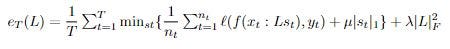
Our goal is to minimize the loss for each task while maximizing the shared information used between tasks. We do so with the objective function e_T we are trying to minimize:

Where ℓ is our chosen loss function.

Essentially, the first clause accounts for our task-specific loss, the second tries to minimize our weight vectors and make them sparse, and our last clause tries to minimize our basis vectors.

**This equation carries two inefficiencies (see if you can figure out what)! Our first is that our equation depends on all previous training data, (specifically the inner sum), which we can imagine is incredibly cumbersome. We alleviate this first inefficiency using a Taylor sum of approximation of the equation. Our second inefficiency is that we need to recompute every s_t to evaluate one instance of L. We eliminate this inefficiency by removing our minimization over z and instead computing s when t is last interacted with. I encourage you to read the original paper for a more detailed explanation!**

Now that we have our objective function, we want to create a method to optimize it!

In training, we’re going to treat each iteration as a unit where we receive a batch of training data from a single task, then compute s_t, and finally update L. At the start of our algorithm, we set T (our number-of-tasks counter), A, b, and L to zeros. Now, for each batch of data, we case based on the data is from a seen or unseen task.

If we encounter data from a new task, we will add 1 to T, and initialize X_t and y_t for this new task, setting them equal to our current batch of X and y..

If we encounter data we’ve already seen, our process gets more complex. We again add our new X and y to add our new X and y to our current memory of X_t and y_t (by running through all data, we will have a complete set of X and y for each task!). We also incrementally update our A and b values negatively (I’ll explain this later, just remember this for now!).

Now we check if we want to end our training loop. We set our (θ_t, D_t) equal to the output of our regular learner for our batch data.

We then check to end the loop (if we have seen all training data). If we haven’t ended, we move on to computing s and updating L.

To compute s, we first compute optimal model theta_t using only the batched data, which will depend on our specific task and loss function.

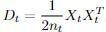
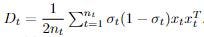
We then compute D_t, and either randomly or to one of the θ_ts initialize any all-zero columns of L (which occurs if a certain basis vector is unused). In linear regression,

and in logistic regression

Then, we compute s_t using L by solving an L1-regularized regression problem:

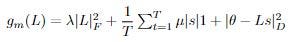
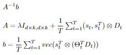
For our final step of updating L, we take

, find where the gradient is 0, then solve for L. By doing so, we increase the sparsity of L! We then output the updated columnwise-vectorization of L as

so as not to sum over all tasks to compute A and b, we construct them incrementally as each task arrives.

Once we’ve iterated through all batch data, we’ve learned all tasks properly and have finished!

The power of ELLA lies in many of its efficiency optimizations, primarily of which is its method of using θ functions to understand exactly what basis knowledge is useful! If you care about a more in-depth understanding of ELLA, I highly encourage you to check out the pseudocode and explanation in the original paper.

Using ELLA as a base, we can imagine creating a generalizable AI, which can learn any task it’s presented with. We again have the property that the more our knowledge basis grows, the more ‘relevant information’ it contains, which will even further increase the speed of learning new tasks! It seems as if ELLA could be the core of one of the super-intelligent artificial learners of the future!

Voyager

What happens when we integrate the newest leap in AI, LLMs, with Lifelong ML? We get something that can beat Minecraft (This is the setting of the actual paper)!

Guanzhi Wang, Yuqi Xie, and others saw the new opportunity offered by the power of GPT-4, and decided to combine it with ideas from lifelong learning you’ve learned so far to create Voyager.

When it comes to learning games, typical algorithms are given predefined final goals and checkpoints for which they exist solely to pursue. In open-world games like Minecraft, however, there are many possible goals to pursue and an infinite amount of space to explore. What if our goal is to approximate human-like self-motivation combined with increased time efficiency in traditional Minecraft benchmarks, such as getting a diamond? Specifically, let’s say we want our agent to be able to decide on feasible, interesting tasks, learn and remember skills, and continue to explore and seek new goals in a ‘self-motivated’ way.

Towards these goals, Wang, Xie, and others created Voyager, which they called the first LLM-powered embodied lifelong learning agent!

How does Voyager work?

On a large-scale, Voyager uses GPT-4 as its main ‘intelligence function’ and the model itself can be separated into three parts:

1. Automatic curriculum: This decides which goals to pursue, and can be thought of as the model’s “motivator”. Implemented with GPT-4, they instructed it to optimize for difficult yet feasible goals and to “discover as many diverse things as possible” (read the original paper to see their exact prompts). If we pass four rounds of our iterative prompting mechanism loop without the agent’s environment changing, we simply choose a new task!
2. Skill library: a collection of executable actions such as craftStoneSword() or getWool() which increase in difficulty as the learner explores. This skill library is represented as a vector database, where keys are embedding vectors of GPT-3.5-generated skill descriptions, and executable skills in code form. GPT-4 generated the code for the skills, optimized for generalizability and refined by feedback from the use of the skill in the agent’s environment!
3. Iterative prompting mechanism: This is the element that interacts with the Minecraft environment. It first executes its’ interface of Minecraft to gain information about its current environment, for example, the items in its inventory and the surrounding creatures it can observe. It then prompts GPT-4 and performs the actions specified in the output, also offering feedback about whether the actions specified are impossible. This repeats until the current task (as decided by the automatic curriculum) is completed. At completion, we add the learned skill to the skill library. For example, if our task was create a stone sword, we now put the skill craftStoneSword() into our skill library. Finally, we ask the automatic curriculum for a new goal.

Now, where does Lifelong Learning fit into all this?

When we encounter a new task, we query our skill database to find the top 5 most relevant skills to the task at hand (for example, relevant skills for the task getDiamonds() would be craftIronPickaxe() and findCave().

Thus, we’ve used previous tasks to learn our new task more efficiently: the essence of lifelong learning! Through this method, Voyager continuously explores and grows, learning new skills that increase its frontier of possibilities, increasing the scale of ambition of its goals, thus increasing the powers of its newly learned skills, continuously!

Compared with other models like AutoGPT, ReAct, and Reflexion, Voyager discovered 3.3x as many new items as these others, navigated distances 2.3x longer, unlocked wooden level 15.3x faster per prompt iteration, and was the only one to unlock the diamond level of the tech tree! Moreover, after training, when dropped in a completely new environment with no items, Voyager consistently solved prior-unseen tasks, while others could not solve any within 50 prompts.

As a display of the importance of Lifelong Learning, without the skill library, the model’s progress in learning new tasks plateaued after 125 iterations, whereas with the skill library, it kept rising at the same high rate!

Now imagine this agent applied to the real world! Imagine a learner with infinite time and infinite motivation that could keep increasing its possibility frontier, learning faster and faster the more prior knowledge it has! I hope by now I’ve properly illustrated the power of Lifelong Machine Learning and its capability to prompt the next transformation of AI!

If you’re interested further in LLML, I encourage you to read Zhiyuan Chen and Bing Liu’s book which lays out the potential future paths LLML might take!

Thank you for making it all the way here! If you’re interested, check out my website anandmaj.com which has my other writing, projects, and art, and follow me on Twitter @almondgod.

Original Papers and other Sources:

Eaton and Ruvolo: Efficient Lifelong Learning Algorithm

Wang, Xie, et al: Voyager

Chen and Liu, Lifelong Machine Learning (Inspired me to write this!): https://www.cs.uic.edu/~liub/lifelong-machine-learning-draft.pdf

Unsupervised LL with Curricula: https://par.nsf.gov/servlets/purl/10310051

Deep LL: https://towardsdatascience.com/deep-lifelong-learning-drawing-inspiration-from-the-human-brain-c4518a2f4fb9

Neuro-inspired AI: https://www.cell.com/neuron/pdf/S0896-6273(17)30509-3.pdf

Embodied LL: https://lis.csail.mit.edu/embodied-lifelong-learning-for-decision-making/

LL for sentiment classification: https://arxiv.org/abs/1801.02808

Lifelong Robot Learning: https://www.sciencedirect.com/science/article/abs/pii/092188909500004Y

Knowledge Basis Idea: https://arxiv.org/ftp/arxiv/papers/1206/1206.6417.pdf

Q-Learning: https://link.springer.com/article/10.1007/BF00992698

AGI LLLM LLMs: https://towardsdatascience.com/towards-agi-llms-and-foundational-models-roles-in-the-lifelong-learning-revolution-f8e56c17fa66

DEPS: https://arxiv.org/pdf/2302.01560.pdf

Voyager: https://arxiv.org/pdf/2305.16291.pdf

Meta-Learning: https://machine-learning-made-simple.medium.com/meta-learning-why-its-a-big-deal-it-s-future-for-foundation-models-and-how-to-improve-it-c70b8be2931b

Meta Reinforcement Learning Survey: https://arxiv.org/abs/2301.08028

Examining Lifelong Machine Learning through ELLA and Voyager: Part 2 of Why LLML is Next in AI was originally published in Towards Data Science on Medium, where people are continuing the conversation by highlighting and responding to this story.

Understanding the power of Lifelong Machine Learning through Q-Learning and Explanation-Based Neural Networks

How does Machine Learning progress from here? Many, if not most, of the greatest innovations in ML have been inspired by Neuroscience. The invention of neural networks and attention-based models serve as prime examples. Similarly, the next revolution in ML will take inspiration from the brain: Lifelong Machine Learning.

Modern ML still lacks humans’ ability to use past information when learning new domains. A reinforcement learning agent who has learned to walk, for example, will learn how to climb from ground zero. Yet, the agent can instead use continual learning: it can apply the knowledge gained from walking to its process of learning to climb, just like how a human would.

Inspired by this property, Lifelong Machine Learning (LLML) uses past knowledge to learn new tasks more efficiently. By approximating continual learning in ML, we can greatly increase the time efficiency of our learners.

To understand the incredible power of LLML, we can start from its origins and build up to modern LLML. In Part 1, we examine Q-Learning and Explanation-Based Neural Networks. In Part 2, we explore the Efficient Lifelong Learning Algorithm and Voyager! I encourage you to read Part 1 before Part 2, though feel free to skip to Part 2 if you prefer!

The Origins of Lifelong Machine Learning

Sebastian Thrun and Tom Mitchell, the fathers of LLML, began their LLML journey by examining reinforcement learning as applied to robots. If the reader has ever seen a visualized reinforcement learner (like this agent learning to play Pokemon), they’ll realize that to achieve any training results in a reasonable human timescale, the agent must be able to iterate through millions of actions (if not much more) over their training period. Robots, though, take multiple seconds to perform each action. As a result, moving typical online reinforcement learning methods to robots results in a significant loss of both the efficiency and capability of the final robot model.

What makes humans so good at real-world learning, where ML in robots is currently failing?

Thrun and Mitchell identified potentially the largest gap in the capabilities of modern ML: its inability to apply past information to new tasks. To solve this issue, they created the first Explanation-Based Neural Network (EBNN), which was the first use of LLML!

To understand how it works, we first can understand how typical reinforcement learning (RL) operates. In RL, our ML model decides the actions of our agent, which we can think of as the ‘body’ that interacts with whatever environment we chose. Our agent exists in environment W with state Z, and when agent takes action A, it receives sensation S (feedback from its environment, for example the position of objects or the temperature). Our environment is a mapping Z x A -> Z (for every action, the environment changes in a specified way). We want to maximize the reward function R: S -> R in our model F: S -> A (in other words we want to choose the action that reaches the best outcome, and our model takes sensation as input and outputs an action). If the agent has multiple tasks to learn, each task has its own reward function, and we want to maximize each function.

We could train each individual task independently. However, Thrun and Michael realized that each task occurs in the same environment with the same possible actions and sensations for our agent (just with different reward functions per task). Thus, they created EBNN to use information from previous problems to solve the current task (LLML)! For example, a robot can use what it’s learned from a cup-flipping task to perform a cup-moving task, since in cup-flipping it has learned how to grab the cup.

To see how EBNN works, we now need to understand the concept of the Q function.

Q* and Q-Learning

Q: S x A -> r is an evaluation function where r represents the expected future total reward after action A in state S. If our model learns an accurate Q, it can simply select the action at any given point that maximizes Q.

Now, our problem reduces to learning an accurate Q, which we call Q*. One such scheme is called Q-Learning, which some think is the inspiration behind OpenAI’s Q* (though the naming might be a complete coincidence).

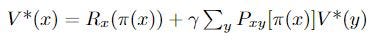
In Q-learning, we define our action policy as function π which outputs an action for each state, and the value of state X as function

Which we can think of as the immediate reward for action π(x) plus the sum of the probabilities of all possible future actions multiplied by their values (which we compute recursively). We want to find the optimal policy (set of actions) π* such that

(at every state, the policy chooses the action that maximizes V*). As the process repeats Q will become more accurate, improving the agent’s selected actions. Now, we define Q* values as the true expected reward for performing action a:

In Q-learning, we reduce the problem of learning π* to the problem of learning the Q*-values of π*. Clearly, we want to choose the actions with the greatest Q-values.

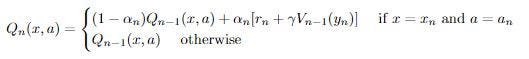
We divide training into episodes. In the nth episode, we get state x_n, select and perform action a_n, observe y_n, receive reward r_n, and adjust Q values using constant α according to:

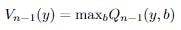
Where

Essentially, we leave all previous Q values the same except for the Q value corresponding to the previous state x and the selected action a. For that Q value, we update it by weighing the previous episode’s Q value by (1 — α) and adding to it our payoff plus the max of the previous episode’s value for the current state y, both weighted by α.

Remember that this algorithm is trying to approximate an accurate Q for each possible action in each possible state. So when we update Q, we update the value for Q corresponding to the old state and the action we took on that episode, since we

The smaller α is, the less we change Q each episode (1 – α will be very large). The larger α is, the less we care about the old value of Q (at α = 1 it is completely irrelevant) and the more we care about what we’ve discovered to be the expected value of our new state.

Let’s consider two cases to gain an intuition for this algorithm and how it updates Q(x, a) after we take action a from state x to reach state y:

1. We go from state x through action a to state y, and are at an ‘end path’ where no more actions are possible. Then, Q(x, a), the expected value for this action and the state before it, should simply be the immediate reward for a (think about why!). Moreover, the higher the reward for a, the more likely we are to choose it in our next episode. Our largest Q value in the previous episode at this state is 0 since no actions are possible, so we are only adding the reward for this action to Q, as intended!
2. Now, our correct Q*s recurse backward from the end! Let’s consider the action b that led from state w to state x, and let’s say we’re now 1 episode later. Now, when we update Q*(w, b), we will add the reward for b to the value for Q*(x, a), since it must be the highest Q value if we chose it before. Thus, our Q(w, b) is now correct as well (think about why)!

Great! Now that you have intuition for Q-learning, we can return to our original goal of understanding:

The Explanation Based Neural Network (EBNN)

We can see that with simple Q-learning, we have no LL property: that previous knowledge is used to learn new tasks. Thrun and Mitchell originated the Explanation Based Neural Network Learning Algorithm, which applies LL to Q-learning! We divide the algorithm into 3 steps.

(1) After performing a sequence of actions, the agent predicts the states that will follow up to a final state s_n, at which no other actions are possible. These predictions will differ from the true observed states since our predictor is currently imperfect (otherwise we’d have finished already)!

(2) The algorithm extracts partial derivatives of the Q function with respect to the observed states. By initially computing the partial derivative of the final reward with respect to the final state s_n, (by the way, we assume the agent is given the reward function R(s)), and we compute slopes backward from the final state using the already computer derivatives using chain rule:

Where M: S x A -> S is our model and R is our final reward.

(3) Now, we’ve estimated the slopes of our Q*s, and we use these in backpropagation to update our Q-values! For those that don’t know, backpropagation is the method through which neural networks learn, where they calculate how the final output of the network changes when each node in the network is changed using this same backward-calculated slope method, and then they adjust the weights and biases of these nodes in the direction that makes the network’s output more desirable (however this is defined by the cost function of the network, which serves the same purpose as our reward function)!

We can think of (1) as the Explaining step (hence the name!), where we look at past actions and try to predict what actions would arise. With (2), we then Analyze these predictions to try to understand how our reward changes with different actions. In (3), we apply this understanding to Learn how to improve our action selection through changing our Qs.

This algorithm increases our efficiency by using the difference between past actions and estimations of past actions as a boost to estimate the efficiency of a certain action path. The next question you might ask is:

How does EBNN help one task’s learning transfer to another?

When we use EBNN applied to multiple tasks, we represent information common between tasks as NN action models, which gives us a boost in learning (a productive bias) through the explanation and analysis process. It uses previously learned, task-independent knowledge when learning new tasks. Our key insight is that we have generalizable knowledge because every task shares the same agent, environment, possible actions, and possible states. The only dependent on each task is our reward function! So by starting from the explanation step with our task-specific reward function, we can use previously discovered states from old tasks as training examples and simply replace the reward function with our current task’s reward function, accelerating the learning process by many fold! The LML fathers discovered a 3 to 4-fold increase in time efficiency for a robot cup-grasping task, and this was only the beginning!

If we repeat this explanation and analysis process, we can replace some of the need for real-world exploration of the agent’s environment required by naive Q-learning! And the more we use it, the more productive it becomes, since (abstractly) there is more knowledge for it to pull from, increasing the likelihood that the knowledge is relevant to the task at hand.

Ever since the fathers of LLML sparked the idea of using task-independent information to learn new tasks, LLML has expanded past not only reinforcement learning in robots but also to the more general ML setting we know today: supervised learning. Paul Ruvolo and Eric Eatons’ Efficient Lifelong Learning Algorithm (ELLA) will get us much closer to understanding the power of LLML!

Please read Part 2: Examining LLML through ELLA and Voyager to see how it works!

Thank you for reading Part 1! Feel free to check out my website anandmaj.com which has my other writing, projects, and art, and follow me on Twitter.

Original Papers and other Sources:

Thrun and Mitchel: Lifelong Robot Learning

Watkins: Q-Learning

Chen and Liu, Lifelong Machine Learning (Inspired me to write this!): https://www.cs.uic.edu/~liub/lifelong-machine-learning-draft.pdf

Unsupervised LL with Curricula: https://par.nsf.gov/servlets/purl/10310051

Deep LL: https://towardsdatascience.com/deep-lifelong-learning-drawing-inspiration-from-the-human-brain-c4518a2f4fb9

Neuro-inspired AI: https://www.cell.com/neuron/pdf/S0896-6273(17)30509-3.pdf

Embodied LL: https://lis.csail.mit.edu/embodied-lifelong-learning-for-decision-making/

EfficientLLA (ELLA): https://www.seas.upenn.edu/~eeaton/papers/Ruvolo2013ELLA.pdf

LL for sentiment classification: https://arxiv.org/abs/1801.02808

Knowledge Basis Idea: https://arxiv.org/ftp/arxiv/papers/1206/1206.6417.pdf

AGI LLLM LLMs: https://towardsdatascience.com/towards-agi-llms-and-foundational-models-roles-in-the-lifelong-learning-revolution-f8e56c17fa66

DEPS: https://arxiv.org/pdf/2302.01560.pdf

Voyager: https://arxiv.org/pdf/2305.16291.pdf

Meta-Learning: https://machine-learning-made-simple.medium.com/meta-learning-why-its-a-big-deal-it-s-future-for-foundation-models-and-how-to-improve-it-c70b8be2931b

Meta Reinforcement Learning Survey: https://arxiv.org/abs/2301.08028

The Origins of Lifelong ML: Part 1 of Why LLML is the Next Game-changer of AI was originally published in Towards Data Science on Medium, where people are continuing the conversation by highlighting and responding to this story.

The art of getting quick gains with agile model production

This post was written together with and inspired by Yuval Cohen

Introduction

Every day, numerous data science projects are discarded due to insufficient prediction accuracy. It’s a regrettable outcome, considering that often these models could be exceptionally well-suited for some subsets of the dataset.

Data Scientists often try to improve their models by using more complex models and by throwing more and more data at the problem. But many times there is a much simpler and more productive approach: Instead of trying to make all of our predictions better all at once, we could start by making good predictions for the easy parts of the data, and only then work on the harder parts.

This approach can greatly affect our ability to solve real-world problems. We start with the quick gain on the easy problems and only then focus our effort on the harder problems.

Thinking Agile

Agile production means focusing on the easy data first, and only after it has been properly modelled, moving on the the more complicated tasks. This allows a workflow that is iterative, value-driven, and collaborative.

It allows for quicker results, adaptability to changing circumstances, and continuous improvement, which are core ideas of agile production.

1. Iterative and incremental approach: work in short, iterative cycles. Start by achieving high accuracy for the easy problems and then move on to the harder parts.
2. Focus on delivering value: work on the problem with the highest marginal value for your time.
3. Flexibility and adaptability: Allow yourself to adapt to changing circumstances. For example, a client might need you to focus on a certain subset of the data — once you’ve solved that small problem, the circumstances have changed and you might need to work on something completely different. Breaking the problem into small parts allows you to adapt to the changing circumstances.
4. Feedback and continuous improvement: By breaking up a problem you allow yourself to be in constant and continuous improvement, rather than waiting for big improvements in large chunks.
5. Collaboration: Breaking the problem into small pieces promotes parallelization of the work and collaboration between team members, rather than putting all of the work on one person.

Breaking down the complexity

In real-world datasets, complexity is the rule rather than the exception. Consider a medical diagnosis task, where subtle variations in symptoms can make the difference between life-threatening conditions and minor ailments. Achieving high accuracy in such scenarios can be challenging, if not impossible, due to the inherent noise and nuances in the data.

This is where the idea of coverage comes into play. Coverage refers to the portion of the data that a model successfully predicts or classifies with high confidence or high precision. Instead of striving for high accuracy across the entire dataset, researchers can choose to focus on a subset of the data where prediction is relatively straightforward. By doing so, they can achieve high accuracy on this subset while acknowledging the existence of a more challenging, uncovered portion.

For instance, consider a trained model with a 50% accuracy rate on a test dataset. In this scenario, it’s possible that if we could identify and select only the predictions we are very sure about (although we should decide what “very sure” means), we could end up with a model that covers fewer cases, let’s say around 60%, but with significantly improved accuracy, perhaps reaching 85%.

I don’t know any product manager who would say no in such a situation. Especially if there is no model in production, and this is the first model.

The two-step model

We want to divide our data into two distinct subsets: the covered and the uncovered. The covered data is the part of the data where the initial model achieves high accuracy and confidence. The uncovered data is the part of the data where our model does not give confident predictions and does not achieve high accuracy.

In the first step, a model is trained on the data. Once we identify a subset of data where the model achieves high accuracy, we deploy that model and let it run on that subset — the covered data.

In the second step, we move our focus to the uncovered data. We try to develop a better model for this data by collecting more data, using more advanced algorithms, feature engineering, and incorporating domain-specific knowledge to find patterns in the data.

At this step, the first thing you should do is look at the errors by eye. Many times you will easily identify many patterns this way before using any fancy tricks.

An example

This example will show how the concept of agile workflow can create great value. This is a very simple example that is meant to visualize this concept. Real-life examples will be a lot less obvious but the idea that you will see here is just as relevant.

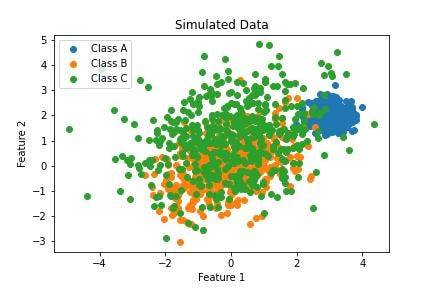
Let’s look at this two-dimensional data that I simulated from three equally sized classes.

num_samples_A = 500
num_samples_B = 500
num_samples_C = 500


# Class A
mean_A = [3, 2]
cov_A = [[0.1, 0], [0, 0.1]]  # Low variance
class_A = np.random.multivariate_normal(mean_A, cov_A, num_samples_A)

# Class B
mean_B = [0, 0]
cov_B = [[1, 0.5], [0.5, 1]]  # Larger variance with some overlap with class C
class_B = np.random.multivariate_normal(mean_B, cov_B, num_samples_B)

# Class C
mean_C = [0, 1]
cov_C = [[2, 0.5], [0.5, 2]]  # Larger variance with some overlap with class B
class_C = np.random.multivariate_normal(mean_C, cov_C, num_samples_C)

Now we try to fit a machine learning classifier to this data, it looks like an SVM classifier with a Gaussian (‘rbf’) kernel might do the trick:

import pandas as pd
from sklearn.model_selection import train_test_split
from sklearn.linear_model import LogisticRegression
from sklearn.svm import SVC

# Creating DataFrame
data = np.concatenate([class_A, class_B, class_C])
labels = np.concatenate([np.zeros(num_samples_A), np.ones(num_samples_B), np.ones(num_samples_C) * 2])
df = pd.DataFrame(data, columns=['x', 'y'])
df['label'] = labels.astype(int)

# Splitting data into train and test sets
X_train, X_test, y_train, y_test = train_test_split(df[['x', 'y']], df['label'], test_size=0.2, random_state=42)

# Training SVM model with RBF kernel
svm_rbf = SVC(kernel='rbf', probability= True)
svm_rbf.fit(X_train, y_train)

# Predict probabilities for each class
svm_rbf_probs = svm_rbf.predict_proba(X_test)

# Get predicted classes and corresponding confidences
svm_rbf_predictions = [(X_test.iloc[i]['x'], X_test.iloc[i]['y'], true_class, np.argmax(probs), np.max(probs)) for i, (true_class, probs) in enumerate(zip(y_test, svm_rbf_probs))]

svm_predictions_df = pd.DataFrame(svm_rbf_predictions).rename(columns={0:'x',1:'y' ,2: 'true_class', 3: 'predicted_class', 4: 'confidence'})

How does this model perform on our data?

accuracy = (svm_predictions_df['true_class'] == svm_predictions_df['predicted_class']).mean()*100
print(f'Accuracy = {round(accuracy,2)}%')

Accuracy = 75.33%

75% percent accuracy is disappointing, but does this mean that this model is useless?

Now we want to look at the most confident predictions and see how the model performs on them. How do we define the most confident predictions? We can try out different confidence (predict_proba) thresholds and see what coverage and accuracy we get for each threshold and then decide which threshold meets our business needs.

thresholds = [.5, .55, .6, .65, .7, .75, .8, .85, .9]
results = []

for threshold in thresholds:
    svm_df_covered = svm_predictions_df.loc[svm_predictions_df['confidence'] > threshold]
    coverage = len(svm_df_covered) / len(svm_predictions_df) * 100
    accuracy_covered = (svm_df_covered['true_class'] == svm_df_covered['predicted_class']).mean() * 100

    results.append({'Threshold': threshold, 'Coverage (%)': round(coverage,2), 'Accuracy on covered data (%)': round(accuracy_covered,2)})

results_df = pd.DataFrame(results)
print(results_df)

And we get

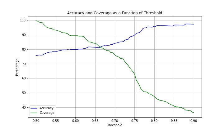
Or if we want a more detailed look we can create a plot of the coverage and accuracy by threshold:

We can now select the threshold that fits our business logic. For example, if our company’s policy is to guarantee at least 90% accuracy, then we can choose a threshold of 0.75 and get an accuracy of 90% for 62% of the data. This is a huge improvement to throwing out the model, especially if we don’t have any model in production!

Now that our model is happily working in production on 60% of the data, we can shift our focus to the rest of the data. We can collect more data, do more feature engineering, try more complex models, or get help from a domain expert.

Balancing act

The two-step model allows us to aim for accuracy while acknowledging that it is perfectly fine to start with a high accuracy for only a subset of the data. It is counterproductive to insist that a model will have high accuracy on all the data before deploying it to production.

The agile approach presented in this post aims for resource allocation and efficiency. Instead of spending computational resources on getting high accuracy all across. Focus your resources on where the marginal gain is highest.

Conclusion

In data science, we try to achieve high accuracy. However, in the reality of messy data, we need to find a clever approach to utilize our resources in the best way. Agile model production teaches us to focus on the parts of the data where our model works best, deploy the model for those subsets, and only then start working on a new model for the more complicated part. This strategy will help you make the best use of your resources in the face of real data science problems.

Think production, Think Agile.

Coverage vs. Accuracy: Striking a Balance in Data Science was originally published in Towards Data Science on Medium, where people are continuing the conversation by highlighting and responding to this story.